###### Nourishment datad_raw_nourishment <-read_xlsx(here("data/raw/PSDS-NC-20240705.xlsx")) |>clean_names() |>mutate(across(where(is.character), ~map_chr(.x, iconv, "UTF-8", "UTF-8", sub=''))) # just in cased_nourishment <- d_raw_nourishment |>mutate(place =str_trim(str_extract(location, "([[:alpha:]][[:space:]]?)+")),place =case_when(str_detect(place, "Topsail") ~"Topsail", place =="Emerald Isle Point"~"Emerald Isle", place =="Cape Hatteras"~"Hatteras Island",.default = place )) |>relocate(place, .after = location) |>mutate(justification =case_match( justification,"Section 111"~"Shore Protection","FEMA Emergency"~"Emergency",.default = justification ))d_rank_n <- d_nourishment |>count(place) |>arrange(desc(n), place) %>%mutate(rank_n =nrow(.) -rank(n, ties.method ="min") +1)d_rank_cy <- d_nourishment |>count(place, wt = volume_cy, name ="cy") |>arrange(desc(cy), place) %>%mutate(rank_n =nrow(.) -rank(cy, ties.method ="min") +1)d_rank_total_cost <- d_nourishment |>count(place, wt = adjusted_cost_2022, name ="total_cost_2022") |>arrange(desc(total_cost_2022), place) %>%mutate(rank_n =nrow(.) -rank(total_cost_2022) +1)###### Location datad_beach_locations <-read_xlsx(here("data/raw/beach-coordinates-geonames-dmoul.xlsx"),skip =3) |>mutate(across(where(is.character), ~map_chr(.x, iconv, "UTF-8", "UTF-8", sub=''))) |># just in casefilter(!is.na(longitude),!is.na(latitude)) |>mutate(place =str_trim(str_to_title(str_extract(place, "([[:alpha:]][[:space:]]?)+"))),place =case_when(str_detect(place, "Topsail") ~"Topsail", place =="Cape Hatteras"~"Hatteras Island", place =="Emerald Isle Point"~"Emerald Isle",str_detect(place, "Figure Eight") ~"Figure Eight Island", # get rid of north end / south end.default = place )) |>distinct(place, .keep_all =TRUE) |>st_as_sf(coords =c("longitude", "latitude"),crs ="WGS84")nc_coast_bbox <-st_bbox(d_beach_locations)d_combined <-left_join(d_beach_locations, d_nourishment,by ="place") |>mutate(primary_funding_source =factor(primary_funding_source, levels =c("Private", "Local", "State", "Federal")) )year_first <-min(d_combined$year_completed)year_last <-max(d_combined$year_completed)n_all_episodes <-nrow(d_combined)d_combined_with_est <- d_combined |>st_drop_geometry() |>mutate(adjusted_cost_2022 =if_else(adjusted_cost_2022 ==0,NA, adjusted_cost_2022),adjusted_cost_cy =if_else(adjusted_cost_cy ==0| adjusted_cost_cy >100,NA, adjusted_cost_cy),length_ft =if_else(length_ft ==0,NA, length_ft) ) |>mutate(med_adjusted_cost_2022 =median(adjusted_cost_2022, na.rm =TRUE),med_adjusted_cost_cy =median(adjusted_cost_cy, na.rm =TRUE),med_length_ft =median(length_ft, na.rm =TRUE),.by = place) |>mutate(adjusted_cost_2022_new = med_adjusted_cost_cy * volume_cy,pct_dif_adjusted_cost_2022_est = adjusted_cost_2022_new / med_adjusted_cost_2022,pct_dif_adjusted_cost_2022 = adjusted_cost_2022_new / adjusted_cost_2022) |># Now choose best cost estimatemutate(adjusted_cost_2022_est =if_else(is.na(adjusted_cost_2022), adjusted_cost_2022_new, adjusted_cost_2022),adjusted_cost_cy_est =if_else(is.na(adjusted_cost_cy), med_adjusted_cost_cy, adjusted_cost_cy),est_cost =if_else(is.na(adjusted_cost_2022),"Y","") ) |># While we're at it, we will need length estimates toomutate(length_ft_est =if_else(is.na(length_ft), med_length_ft, length_ft),est_length =if_else(is.na(length_ft),"Y",""), )n_episodes <-nrow(d_combined)n_episodes_cost_missing <- d_combined_with_est |>filter(is.na(adjusted_cost_2022)) |>nrow()pct_episodes_missing_cost <-percent(n_episodes_cost_missing / n_episodes)my_caption_missing_append <-glue("Estimated episode costs for {n_episodes_cost_missing}", " of {n_episodes} episodes ({pct_episodes_missing_cost})","\nindicated by the rug marks at bottom of plot")my_caption_missing_length_append <-glue("Includes estimated episode lengths where data is missing")volume_at_80pct <-quantile(d_combined$volume_cy, na.rm =TRUE,probs =0.8)length_at_80pct <-quantile(d_combined_with_est$length_ft_est, na.rm =TRUE,probs =0.8)##### County boundaries# v2020 <- tidycensus::load_variables(year = 2020,# dataset = "pl")d_raw_county <- tidycensus::get_decennial(geography ="county",variables ="P1_001N",year =2020,state ="NC",geometry =TRUE) |>st_transform(crs ="WGS84")###### Coastlined_nc_border <-st_union(d_beach_locations)fname <-here("data/raw/noaa-shoreline/gshhg-shp-2.3.7/GSHHS_shp/h/")d_raw_h1 <-st_read(fname,layer ="GSHHS_h_L1",quiet =TRUE)d_raw_h2 <-st_read(fname,layer ="GSHHS_h_L2",quiet =TRUE)bbox_eps <-0.1# degreesmy_xmin =min(st_coordinates(d_nc_border)[, 1]) - bbox_epsmy_xmax =max(st_coordinates(d_nc_border)[, 1]) +100* bbox_epsmy_ymin =min(st_coordinates(d_nc_border)[, 2]) -10* bbox_epsmy_ymax =max(st_coordinates(d_nc_border)[, 2]) + bbox_epsplot_bbox <-st_bbox(c(xmin = my_xmin, xmax = my_xmax, ymax = my_ymax, ymin = my_ymin), crs =st_crs("WGS84") )plot_bbox <-st_bbox(c(xmin =-79, xmax =-70, ymax =36.8, ymin =32), crs =st_crs("WGS84") )nc_coastline <-st_crop(d_raw_h1, plot_bbox)# nc_rivers <- st_crop(d_raw_h2, plot_bbox) # doesn't include enough river data for NCnc_counties <-st_crop(d_raw_county, plot_bbox)###### Countsd_combined_count <-count(d_combined, place)d_combined_volume_cy <- d_combined |>filter(!is.na(volume_cy)) |>count(place, wt = volume_cy,name ="total_volume_cy")n_missing_costs <- d_combined |>filter(adjusted_cost_2022 ==0) |>nrow()
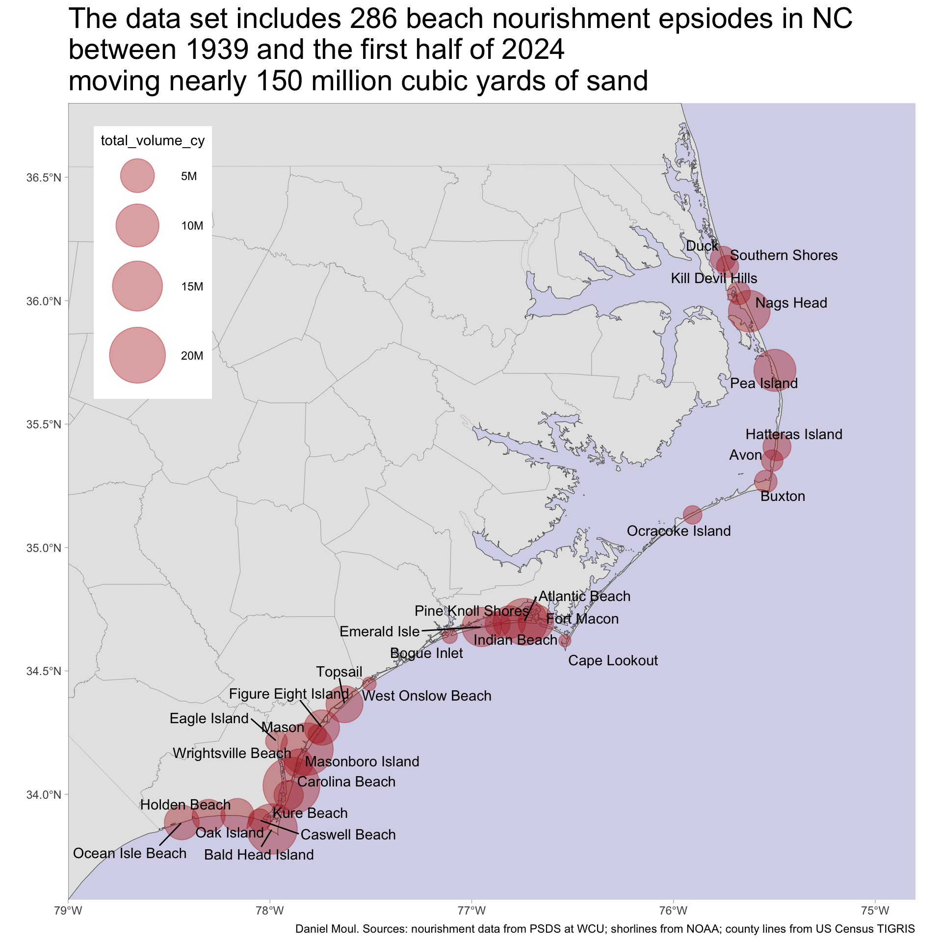
The data set includes 286 nourishment episodes on or near ocean shorelines in North Carolina from 1939 through sometime in the first half of 2024 (I downloaded the data on 2024-07-05). While the costs for a minority of episodes (106, 37%) are not in the data set, the cumulative cost in 2022 dollars for the events that include costs is $1.3B. Using estimates for the missing costs, I estimate the cumulative cost to be $1.6B.
1.1 How much sand, how much money, and with what justifications?
Episodes were distributed along nearly the whole length of NC coastline. Carolina Beach, one of the older beach communities, received 32 nourishment episodes delivering over 20M cubic yards–more than any other place. See the summary Table 1.1.1
1.1.1 Volume of beach nourishment episodes
Show the code
d_combined_volume_cy |>ggplot() +geom_sf(data = nc_coastline,alpha =1) +geom_sf(data = nc_counties,linewidth =0.05,color ="grey40",fill =NA,alpha =0.1) +geom_sf(aes(size = total_volume_cy), color ="firebrick",alpha =0.4) +geom_text_repel(aes(label = place, geometry = geometry),stat ="sf_coordinates",min.segment.length =1,force =20,max.overlaps =20,seed =9999 ) +coord_sf(xlim =c(NA, -74.8)) +scale_x_continuous(expand =expansion(mult =c(0, 0))) +scale_y_continuous(expand =expansion(mult =c(0, 0))) +scale_size_continuous(range =c(4, 20),labels =label_number(scale_cut =cut_short_scale()) ) +guides(size =guide_legend(position ="inside")) +theme(axis.title =element_blank(),panel.border =element_blank(),panel.background =element_rect(fill ="#00008B33"),legend.position.inside =c(0.1, 0.8),legend.key =element_rect(fill ="white"),legend.background =element_rect(fill ="white"),) +labs(title =glue("The data set includes {n_all_episodes} beach nourishment epsiodes in NC", "\nbetween {year_first} and the first half of {year_last}","\nmoving nearly {round(sum(d_combined_volume_cy$total_volume_cy) / 1e6)} million cubic yards of sand"),caption = my_caption_geo )
Figure 1.1: NC beach nourishment map
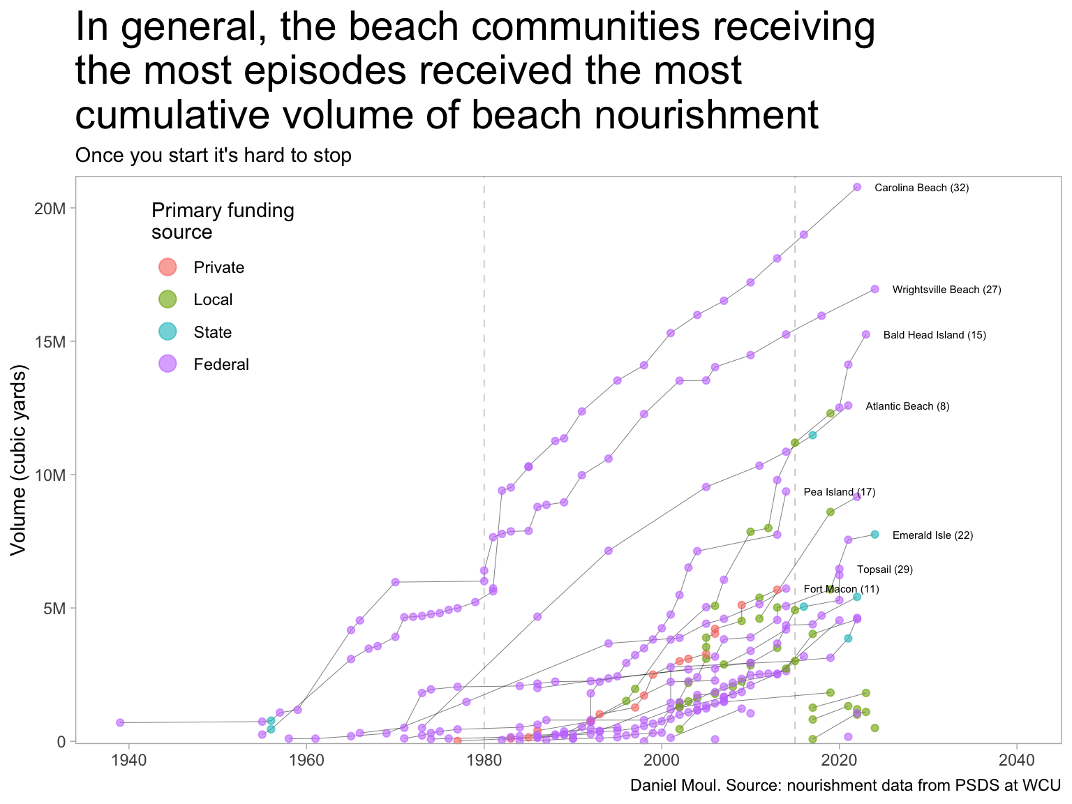
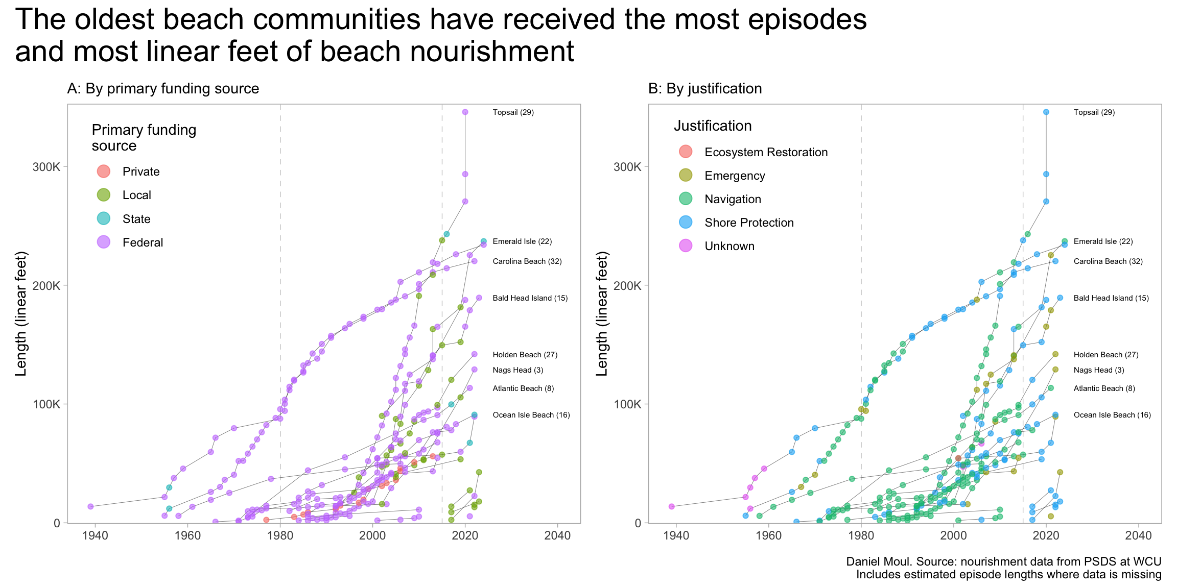
I distinguish three three location clusters by their first beach nourishment episode as seen in Figure 1.2:
Some early beach communities started nourishment before 1980 including Carolina Beach, Wrightsville Beach, and Atlantic Beach
The majority started nourishment in the eighties, nineties or early 2000s
Some places started nourishment since 2018, mainly funded locally, and probably at least in part in response to Hurricane Florence
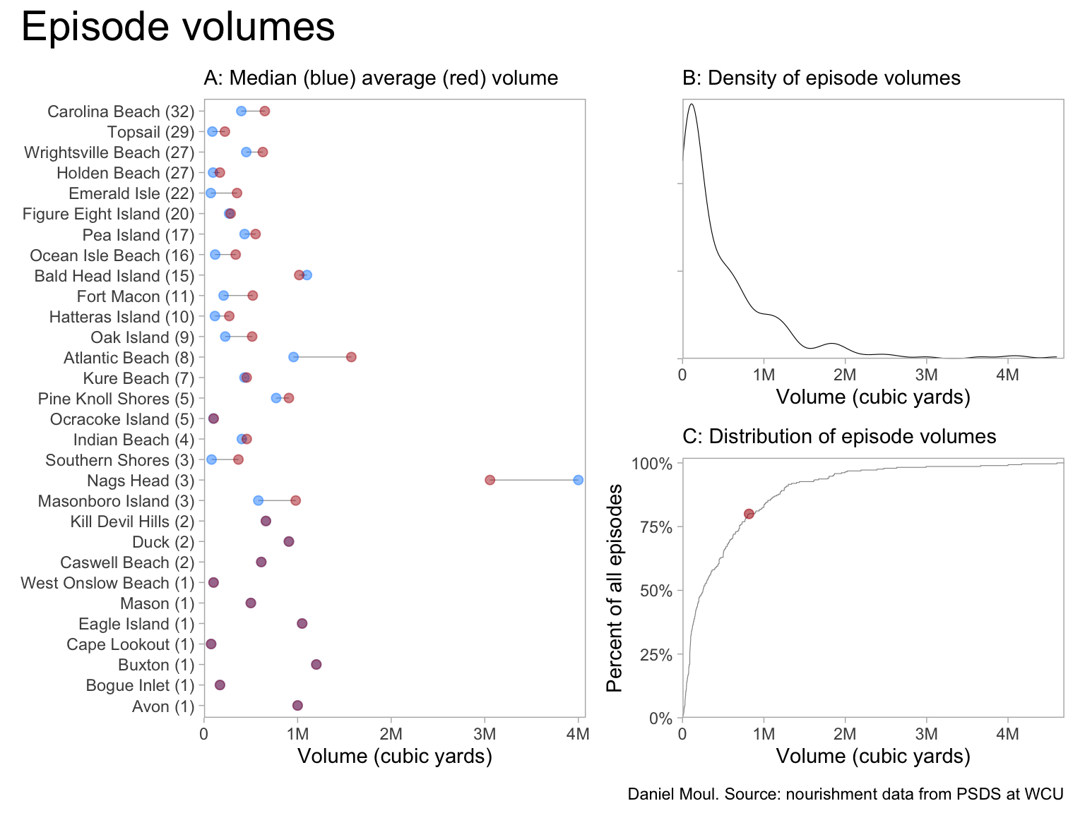
Figure 1.4: Volume per episode with median and average volume for each place
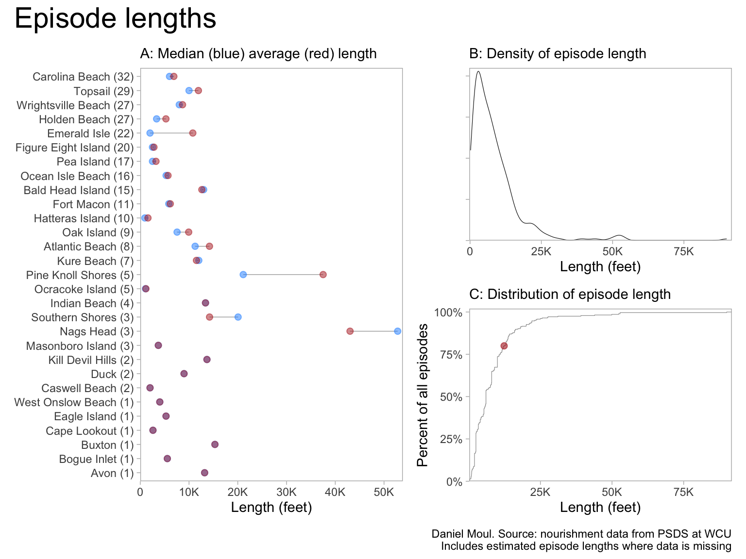
1.1.2 Length of beach nourishment episodes
Eighty percent of the episodes delivered nourishment along less than about 12K linear feet, which is 2.3 miles (panel C). Nags Head and Pine Knoll Shores are notable outliers (panel A).
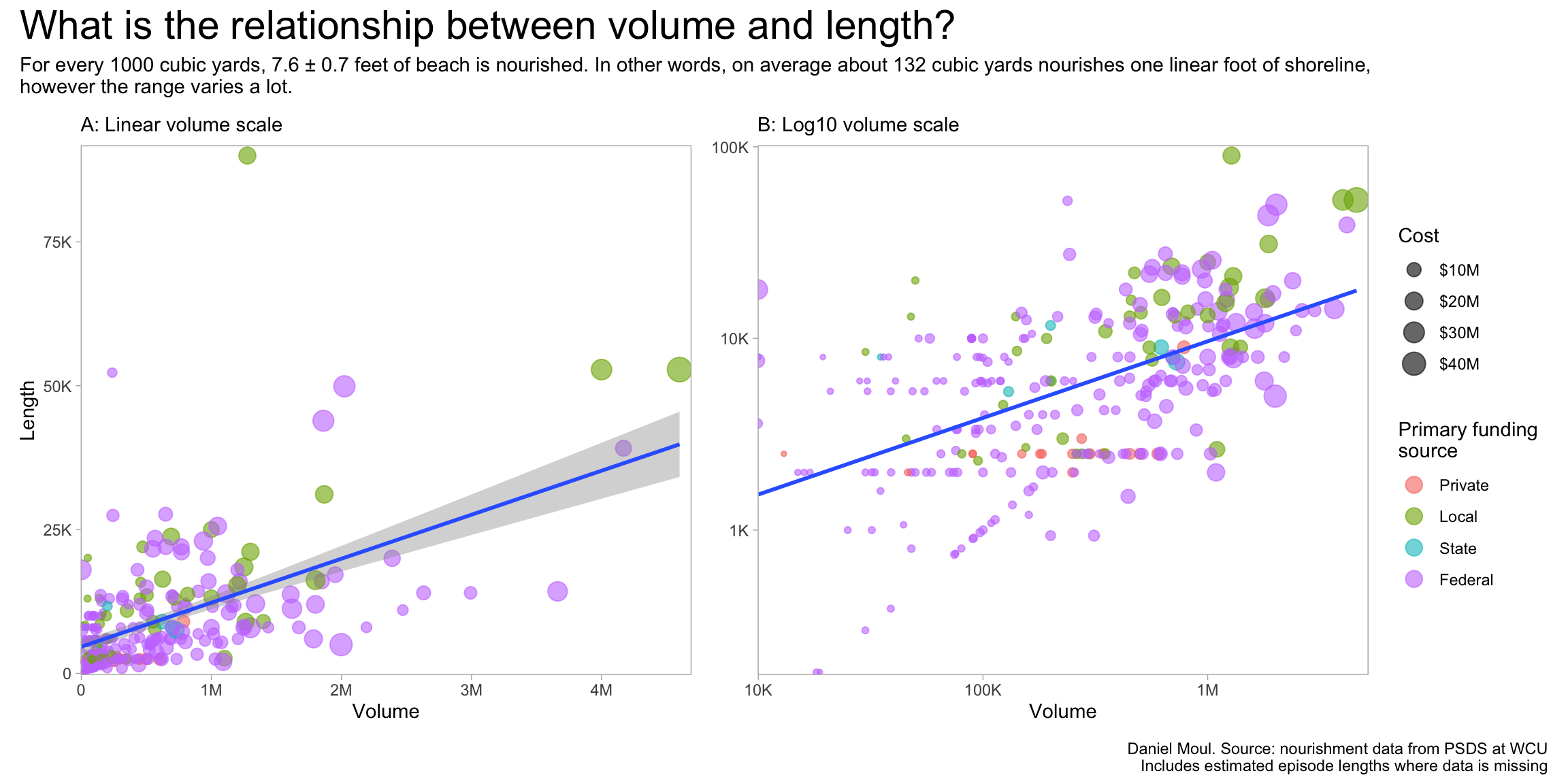
There is a wide range of nourishment lengths and volumes–and their ratios (Figure 1.7). At some locations (example: Carolina Beach) there have been episodes of widely varying volume deposited on very similar lengths of beach while at other locations (example: Topsail beaches) it’s the reverse. See Table 1.1.
Show the code
model1 <- d_combined_with_est |>mutate(volume_cyk = volume_cy /1000) |>lm(length_ft_est ~ volume_cyk,data = _) |> broom::tidy()model1_estimate <-round(model1[2, 2], digits =1)model1_std_error <-round(model1[2, 3], digits =1)one_ft_volume <-round(1000/ model1_estimate)p1 <- d_combined_with_est |>st_drop_geometry() |>mutate(primary_funding_source =factor(primary_funding_source, levels =c("Private", "Local", "State", "Federal")) ) |>ggplot(aes(x = volume_cy, y = length_ft_est)) +geom_point(aes(size = adjusted_cost_2022_est,color = primary_funding_source),alpha =0.6,show.legend =TRUE) +geom_smooth(method ='lm', formula ='y ~ x', se =TRUE,span =0.95) +scale_x_continuous(labels =label_number(scale_cut =cut_short_scale()),expand =expansion(mult =c(0.001, 0.02))) +scale_y_continuous(labels =label_number(scale_cut =cut_short_scale()),expand =expansion(mult =c(0.005, 0.02))) +scale_size_continuous(labels =label_dollar(scale_cut =cut_short_scale())) +guides(color ="none") +labs(subtitle ="A: Linear volume scale",x ="Volume",y ="Length",size ="Cost",color ="Primary funding\nsource" )p2 <- d_combined_with_est |>st_drop_geometry() |>mutate(primary_funding_source =factor(primary_funding_source, levels =c("Private", "Local", "State", "Federal")) ) |>ggplot(aes(x = volume_cy, y = length_ft_est)) +geom_point(aes(size = adjusted_cost_2022_est,color = primary_funding_source),alpha =0.6,show.legend =TRUE) +geom_smooth(method ='lm', formula ='y ~ x', se =FALSE,span =0.95) +scale_x_log10(labels =label_number(scale_cut =cut_short_scale()),expand =expansion(mult =c(0.001, 0.02))) +scale_y_log10(labels =label_number(scale_cut =cut_short_scale()),expand =expansion(mult =c(0.005, 0.02))) +scale_size_continuous(labels =label_dollar(scale_cut =cut_short_scale())) +guides(color =guide_legend(override.aes =list(size =4))) +labs(subtitle ="B: Log10 volume scale",x ="Volume",y =NULL,size ="Cost",color ="Primary funding\nsource" )p1 + p2 +plot_annotation(title ="What is the relationship between volume and length?",subtitle =glue("For every 1000 cubic yards, {model1_estimate} ± {model1_std_error} feet of beach is nourished."," In other words, on average about {one_ft_volume} cubic yards nourishes one linear foot of shoreline,","\nhowever the range varies a lot."),caption =paste0(my_caption, "\n", my_caption_missing_length_append) ) +plot_layout(guides ="collect" )
Figure 1.7: The relationship of length of shoreline nourished by volume
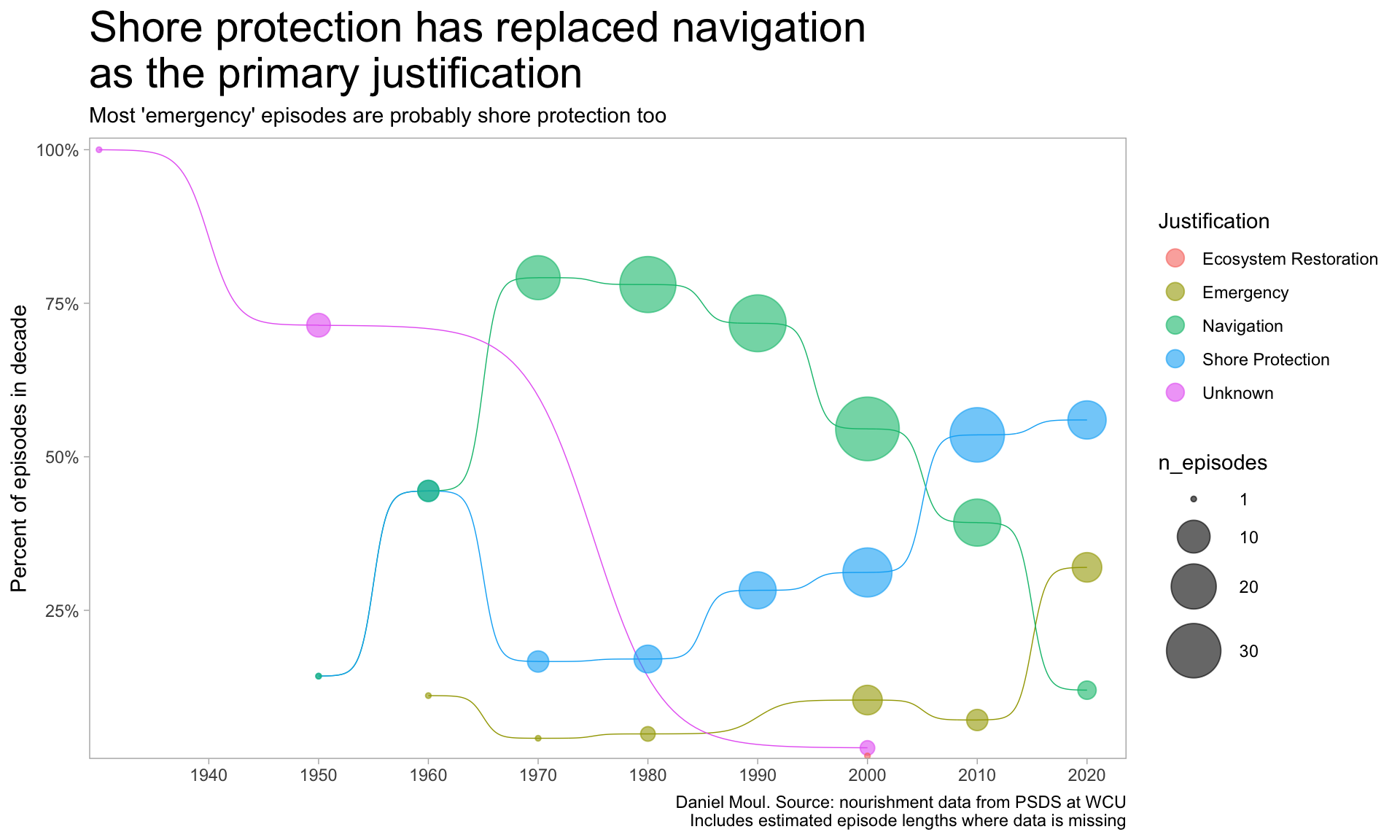
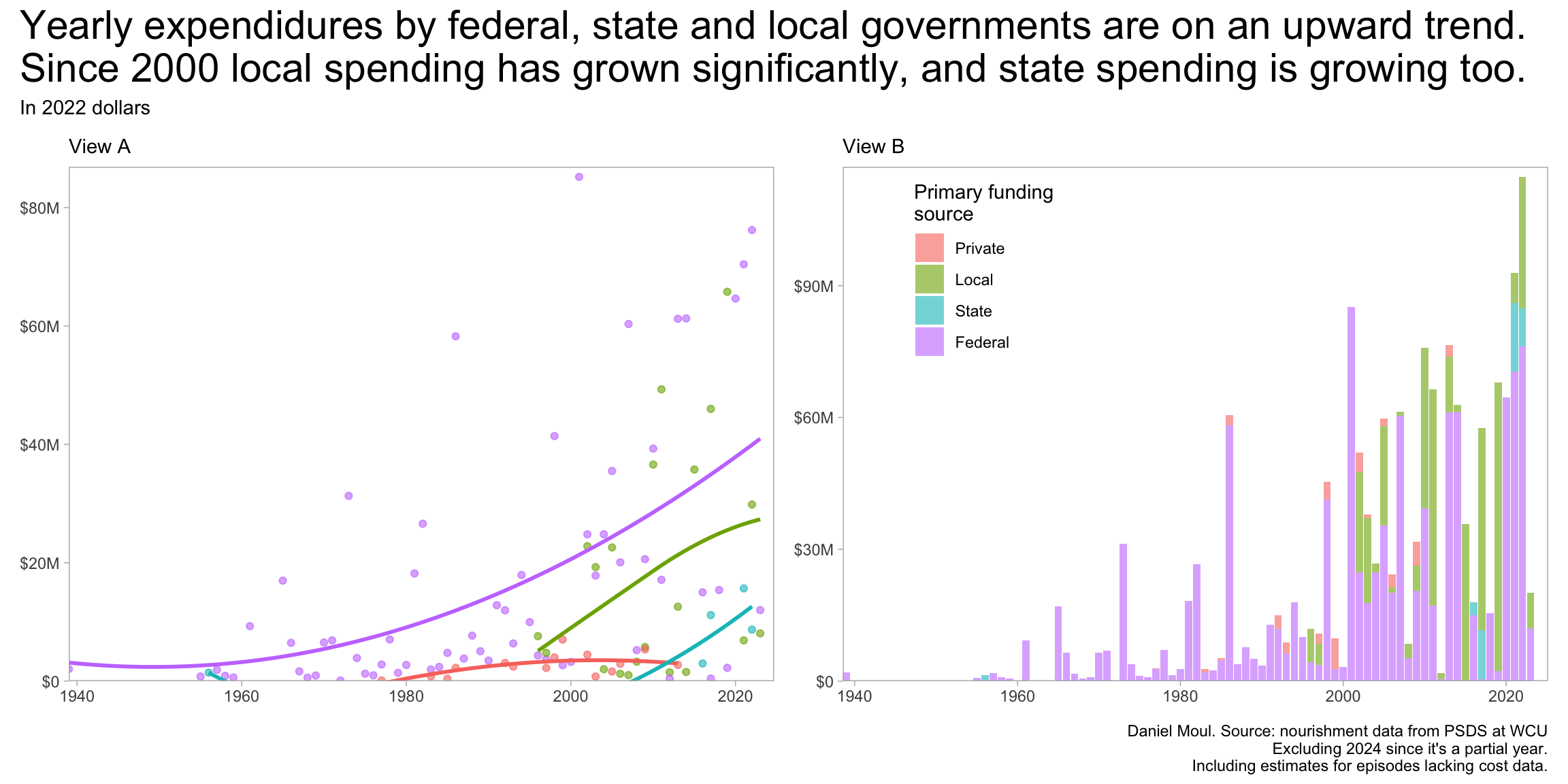
The mix of justifications has shifted from mostly navigation to mostly shore protection.
dta_for_plot <- d_combined_with_est |>filter(year_completed <2024) |># remove partial yeararrange(year_completed) |>summarize(cost =sum(adjusted_cost_2022_est),.by =c(year_completed, primary_funding_source)) |>mutate(primary_funding_source =factor(primary_funding_source, levels =c("Private", "Local", "State", "Federal")) )p1 <- dta_for_plot |>ggplot(aes(x = year_completed, y = cost, color = primary_funding_source)) +geom_point(alpha =0.6,show.legend =FALSE) +geom_smooth(se =FALSE, method ='loess', formula ='y ~ x', span =3.5,alpha =0.6,show.legend =FALSE) +scale_x_continuous(expand =expansion(mult =c(0, 0.02))) +scale_y_continuous(labels =label_dollar(scale_cut =cut_short_scale()),expand =expansion(mult =c(0, 0.02))) +guides(color =guide_legend(override.aes =list(linewidth =3))) +coord_cartesian(clip ="on", ylim =c(0, NA)) +expand_limits(y =0) +labs(subtitle ="View A",x =NULL,y =NULL,color ="Primary funding\nsource" )p2 <- dta_for_plot |>ggplot(aes(x = year_completed, y = cost)) +geom_col(aes(fill = primary_funding_source),alpha =0.6,show.legend =TRUE) +scale_x_continuous(expand =expansion(mult =c(0, 0.02))) +scale_y_continuous(labels =label_dollar(scale_cut =cut_short_scale()),expand =expansion(mult =c(0, 0.02))) +guides(color =guide_legend(override.aes =list(linewidth =3))) +coord_cartesian(clip ="on", ylim =c(0, NA)) +expand_limits(y =0) +guides(fill =guide_legend(position ="inside")) +theme(legend.position.inside =c(0.2, 0.8)) +labs(subtitle ="View B",x =NULL,y =NULL,fill ="Primary funding\nsource" )p1 + p2 +plot_annotation(title =glue("Yearly expendidures by federal, state and local governments are on an upward trend.", "\nSince 2000 local spending has grown significantly, and state spending is growing too."),subtitle =glue("In 2022 dollars"), caption =paste0(my_caption, "\n", "Excluding 2024 since it's a partial year.", "\n", "Including estimates for episodes lacking cost data.") )
Figure 1.9: Yearly cost by primary funding sources
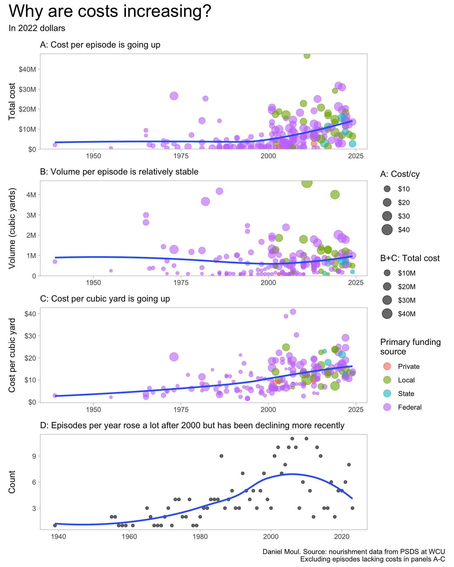
The cost per episode is going up (A), however this is not due to growth in the volume of episodes (B); rather it’s due to an increase in cost per cubic yard (C). If number of episodes per year (D) had not declined in the latest years, overall costs would be higher (see Figure 1.12).
Is the cost per volume increasing, because nourishment projects undertaken in recent years are more challenging (for example: greater distances between dredging and beaches)? Or are environmental regulations more expensive to comply with? Or is there limited competition among a small set of contractors bidding on nourishment projects? Or other reasons?
And why have the number of episodes per year declined in the most recent years? Perhaps because a major hurricane has not hit NC since Florence in 2018. Are there other reasons?
Show the code
p1 <- d_combined |>st_drop_geometry() |>filter(adjusted_cost_2022 >0, adjusted_cost_cy <100) |>mutate(primary_funding_source =factor(primary_funding_source, levels =c("Private", "Local", "State", "Federal")) ) |>ggplot(aes(x = year_completed, y = adjusted_cost_2022)) +geom_point(aes(size = adjusted_cost_cy,color = primary_funding_source),alpha =0.6,show.legend =TRUE) +geom_smooth(method ='loess', formula ='y ~ x', se =FALSE,span =0.95) +scale_y_continuous(labels =label_dollar(scale_cut =cut_short_scale()),expand =expansion(mult =c(0.005, 0.02))) +scale_size_continuous(labels =label_dollar(scale_cut =cut_short_scale())) +guides(color ="none") +labs(subtitle ="A: Cost per episode is going up",x =NULL,y ="Total cost",size ="A: Cost/cy",color ="Primary funding\nsource" )p2 <- d_combined |>st_drop_geometry() |>filter(adjusted_cost_2022 >0, adjusted_cost_cy <100) |>mutate(primary_funding_source =factor(primary_funding_source, levels =c("Private", "Local", "State", "Federal")) ) |>ggplot(aes(x = year_completed, y = volume_cy)) +geom_point(aes(size = adjusted_cost_2022,color = primary_funding_source),alpha =0.6,show.legend =TRUE) +geom_smooth(method ='loess', formula ='y ~ x', se =FALSE,span =0.95) +scale_y_continuous(labels =label_number(scale_cut =cut_short_scale()),expand =expansion(mult =c(0.005, 0.02))) +scale_size_continuous(labels =label_dollar(scale_cut =cut_short_scale())) +guides(color ="none") +labs(subtitle ="B: Volume per episode is relatively stable",x =NULL,y ="Volume (cubic yards)",size ="B+C: Total cost",color ="Primary funding\nsource" )p3 <- d_combined |>st_drop_geometry() |>filter(adjusted_cost_2022 >0, adjusted_cost_cy <100) |>mutate(primary_funding_source =factor(primary_funding_source, levels =c("Private", "Local", "State", "Federal")) ) |>ggplot(aes(x = year_completed, y = adjusted_cost_cy)) +geom_point(aes(size = adjusted_cost_2022,color = primary_funding_source),alpha =0.6) +geom_smooth(method ='loess', formula ='y ~ x', se =FALSE,span =0.95) +scale_y_continuous(labels =label_dollar()) +scale_size_continuous(labels =label_dollar(scale_cut =cut_short_scale())) +guides(color =guide_legend(override.aes =list(size =4))) +labs(subtitle ="C: Cost per cubic yard is going up",x =NULL,y ="Cost per cubic yard",size ="B+C: Total cost",color ="Primary funding\nsource" )p4 <- d_combined_with_est |>count(year_completed) |>filter(year_completed <2024) |># remove partial yearggplot(aes(x = year_completed, y = n)) +geom_point(alpha =0.6) +geom_smooth(method ='loess', formula ='y ~ x', se =FALSE, ) +labs(subtitle ="D: Episodes per year rose a lot after 2000 but has been declining more recently",x =NULL,y ="Count" )p1 / p2 / p3 + p4 +plot_annotation(title ="Why are costs increasing?",subtitle ="In 2022 dollars",caption =paste0(my_caption, "\n", "Excluding episodes lacking costs in panels A-C") ) +plot_layout(guides ="collect" )
Figure 1.10: Why costs have increased explained in four panels
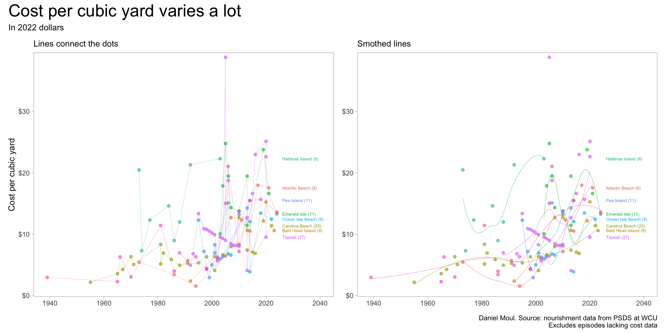
It’s not simply the case that some places are just more expensive per unit volume.
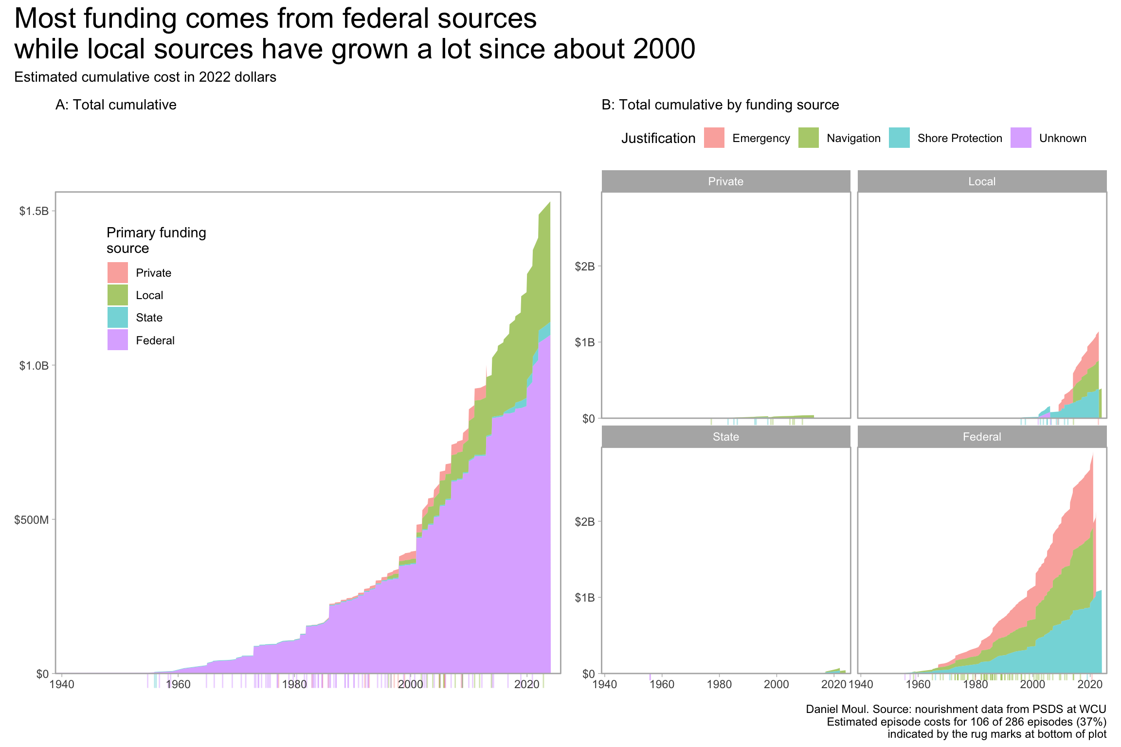
Private and state funders have been bit players. Will state expenditures continue to grow on current trend (Figure 1.9, Figure 1.13) in the years ahead? Should residents in the rest of the state pay for beach nourishment projects, which typically have only short term benefits, even though residents throughout the state (and beyond) travel to the beaches for vacation? Some level of investment can be justified on economic terms–the coastal economy is based on tourism–but how much?
Show the code
d_not_included <- d_combined |>filter(adjusted_cost_2022 ==0) |>mutate(cum_cost =0)dta_for_plot <- d_combined_with_est |>arrange(year_completed) |>mutate(cum_cost =cumsum(adjusted_cost_2022_est),.by = primary_funding_source) |>mutate(primary_funding_source =factor(primary_funding_source, levels =c("Private", "Local", "State", "Federal")) )p1 <- dta_for_plot |>ggplot(aes(x = year_completed, y = cum_cost)) +geom_area(aes(fill = primary_funding_source),alpha =0.6) +geom_rug(data = d_not_included,aes(x = year_completed, y = cum_cost, color = primary_funding_source),sides ="b",outside =TRUE,alpha =0.3,position =position_jitter(),show.legend =FALSE) +scale_x_continuous(expand =expansion(mult =c(0, 0.02))) +scale_y_continuous(labels =label_dollar(scale_cut =cut_short_scale()),expand =expansion(mult =c(0, 0.02))) +guides(fill =guide_legend(position ="inside")) +coord_cartesian(clip ="off") +theme(legend.position.inside =c(0.2, 0.8)) +labs(subtitle ="A: Total cumulative", x =NULL,y =NULL,fill ="Primary funding\nsource" )p2 <- dta_for_plot |>ggplot(aes(x = year_completed, y = cum_cost)) +geom_area(aes(fill = justification),alpha =0.6,show.legend =TRUE) +geom_rug(data = d_not_included,aes(x = year_completed, y = cum_cost, color = justification),sides ="b",outside =TRUE,alpha =0.3,position =position_jitter(),show.legend =FALSE) +scale_x_continuous(expand =expansion(mult =c(0, 0.02))) +scale_y_continuous(labels =label_dollar(scale_cut =cut_short_scale()),expand =expansion(mult =c(0, 0.02))) +facet_wrap( ~primary_funding_source) +coord_cartesian(clip ="off") +theme(legend.position ="top") +labs(subtitle ="B: Total cumulative by funding source", x =NULL,y =NULL,color ="Justification",fill ="Justification" )p1 + p2 +plot_annotation(title =glue("Most funding comes from federal sources","\nwhile local sources have grown a lot since about 2000"),subtitle =glue("Estimated cumulative cost in 2022 dollars"),caption =paste0(my_caption, "\n", my_caption_missing_append) )
Figure 1.12: Cumulative cost by primary funding sources
The relatively small amounts of state funding have gone to different communities each time:
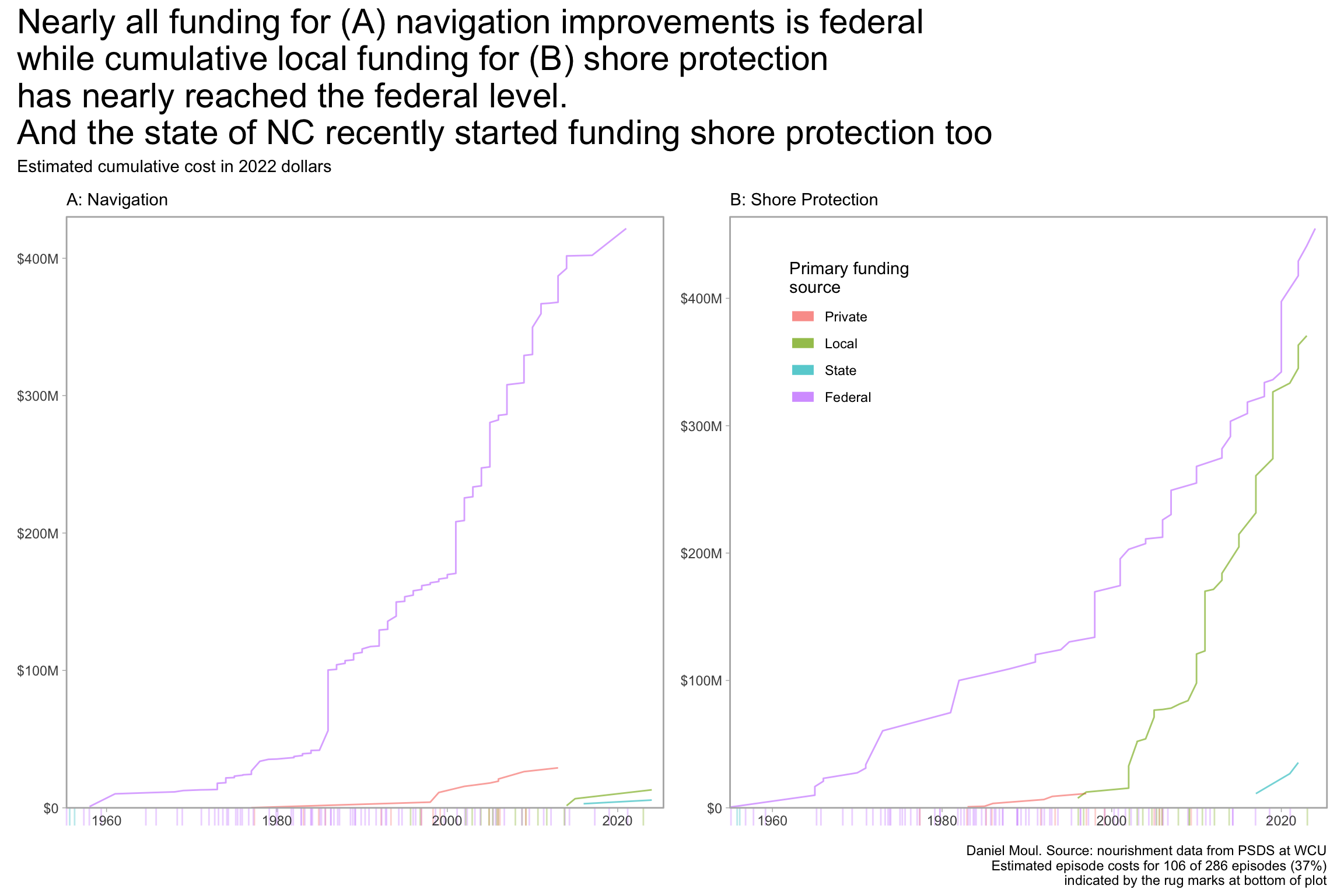
It makes sense to me that the federal government is funding navigation improvements, since it has constitutional obligations related to interstate commerce and the regulation of waterways.
More surprising is the growth of locally-funded shore protection episodes, which in 30 years has nearly reached what the federal government spent in the last 80 years. Can this continue? What stress is this putting on local community budgets and balance sheets? How are they paying for it? Will the trend continue? What if communities reach their capacity to spend?
Show the code
d_not_included <- d_combined |>filter(adjusted_cost_2022 ==0) |>mutate(cum_cost =0)dta_for_plot <- d_combined_with_est |>arrange(year_completed) |>mutate(cum_cost =cumsum(adjusted_cost_2022_est),.by =c(justification, primary_funding_source)) |>mutate(primary_funding_source =factor(primary_funding_source,levels =c("Private", "Local", "State", "Federal")) )p1 <- dta_for_plot |>filter(justification =="Navigation") |>ggplot(aes(x = year_completed, y = cum_cost)) +geom_line(aes(fill = primary_funding_source, color = primary_funding_source, group = primary_funding_source),alpha =0.6,show.legend =FALSE) +geom_rug(data = d_not_included,aes(x = year_completed, y = cum_cost, color = primary_funding_source),sides ="b",outside =TRUE,alpha =0.3,position =position_jitter(),show.legend =FALSE) +scale_x_continuous(expand =expansion(mult =c(0, 0.02))) +scale_y_continuous(labels =label_dollar(scale_cut =cut_short_scale()),expand =expansion(mult =c(0, 0.02))) +coord_cartesian(clip ="off") +labs(subtitle ="A: Navigation", x =NULL,y =NULL,fill ="Primary funding\nsource", )p2 <- dta_for_plot |>filter(justification =="Shore Protection") |>ggplot(aes(x = year_completed, y = cum_cost)) +geom_line(aes(fill = primary_funding_source, color = primary_funding_source, group = primary_funding_source),alpha =0.6) +geom_rug(data = d_not_included,aes(x = year_completed, y = cum_cost, color = primary_funding_source),sides ="b",outside =TRUE,alpha =0.3,position =position_jitter()) +scale_x_continuous(expand =expansion(mult =c(0, 0.02))) +scale_y_continuous(labels =label_dollar(scale_cut =cut_short_scale()),expand =expansion(mult =c(0, 0.02))) +coord_cartesian(clip ="off") +guides(color =guide_legend(position ="inside",override.aes =list(linewidth =3))) +theme(legend.position.inside =c(0.2, 0.8)) +labs(subtitle ="B: Shore Protection", x =NULL,y =NULL,color ="Primary funding\nsource" )p1 + p2 +plot_annotation(title =glue("Nearly all funding for (A) navigation improvements is federal","\nwhile cumulative local funding for (B) shore protection", "\nhas nearly reached the federal level.", "\nAnd the state of NC recently started funding shore protection too"),subtitle =glue("Estimated cumulative cost in 2022 dollars"), caption =paste0(my_caption, "\n", my_caption_missing_append) )
Figure 1.13: Cumulative cost for shore protection and navigation
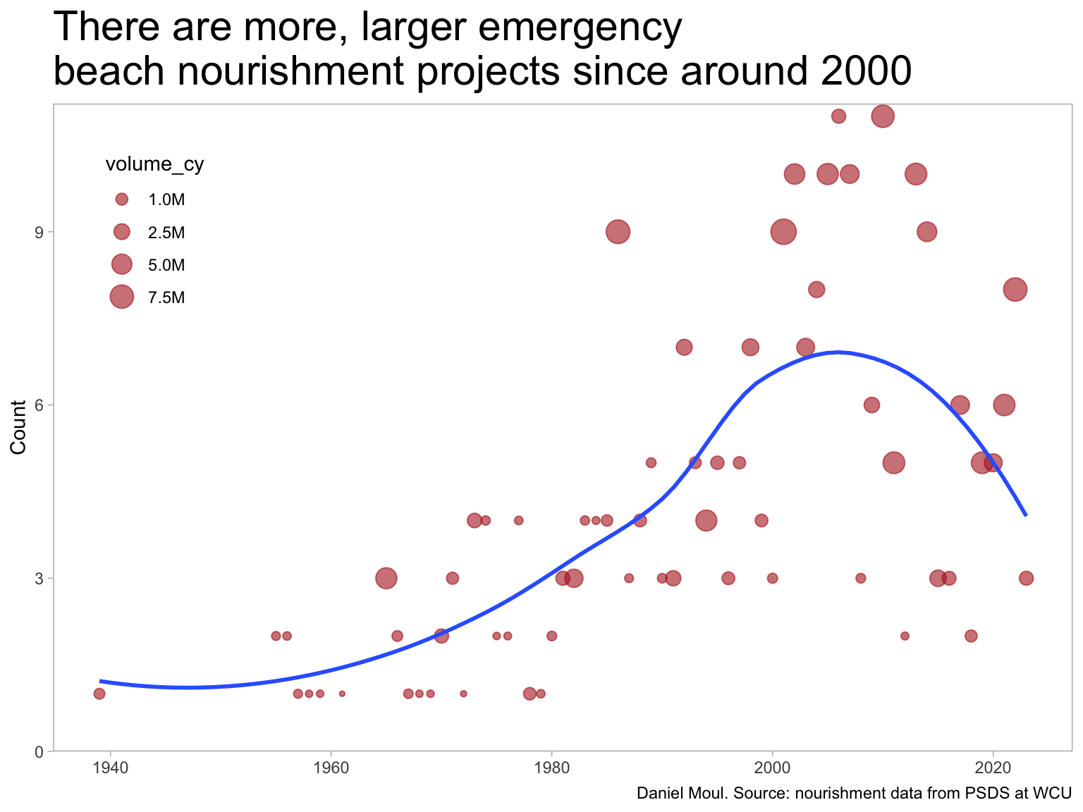
The number of “emergency” episodes has been increasing too.
Table 1.1: All places and episodes with volume and length distributions for each place
All places and episodes with distribution of volume (cubic yards) and length (feet) for each place’s episodes
place
n_episodes
volume_cy
length_ft
volume_cy_dist
length_ft_dist
Carolina Beach
32
20.8M
220K
Topsail
29
6.5M
346K
Wrightsville Beach
27
17.0M
234K
Holden Beach
27
4.6M
142K
Emerald Isle
22
7.8M
237K
Figure Eight Island
20
5.7M
56K
Pea Island
17
9.4M
55K
Ocean Isle Beach
16
5.4M
91K
Bald Head Island
15
15.3M
189K
Fort Macon
11
5.7M
68K
Hatteras Island
10
2.7M
16K
Oak Island
9
4.6M
89K
Atlantic Beach
8
12.6M
114K
Kure Beach
7
3.2M
81K
Pine Knoll Shores
5
4.5M
188K
Ocracoke Island
5
0.5M
6K
Indian Beach
4
1.8M
54K
Nags Head
3
9.2M
129K
Masonboro Island
3
2.9M
11K
Southern Shores
3
1.1M
43K
Duck
2
1.8M
18K
Kill Devil Hills
2
1.3M
27K
Caswell Beach
2
1.2M
4K
Buxton
1
1.2M
15K
Eagle Island
1
1.0M
5K
Avon
1
1.0M
13K
Mason
1
0.5M
0K
Bogue Inlet
1
0.2M
6K
West Onslow Beach
1
0.1M
4K
Cape Lookout
1
0.1M
3K
Total
286
149.6M
2,462K
For those figures in which I estimated costs for one or more episodes (Figure 1.12, Figure 1.13) there is more detail below. The episodes missing costs were below average volume for nearly all places.
Table 1.2: Places with episodes that don’t include costs
Places with at least one episode missing cost data
place
Episodes missing costs
All episodes for place
Percent missing
n_episodes
volume_cy
total_n_episodes
total_volume_cy
pct_episodes
pct_volume
Holden Beach
22
2,115,040
27
4,575,242
81.5%
46.2%
Figure Eight Island
17
4,794,679
20
5,685,251
85%
84.3%
Carolina Beach
12
1,113,111
32
20,783,368
37.5%
5.4%
Emerald Isle
11
434,000
22
7,756,286
50%
5.6%
Wrightsville Beach
11
1,322,416
27
16,956,391
40.7%
7.8%
Ocean Isle Beach
7
311,785
16
5,415,985
43.8%
5.8%
Bald Head Island
6
4,179,800
15
15,256,300
40%
27.4%
Pea Island
6
2,733,307
17
9,367,902
35.3%
29.2%
Fort Macon
4
507,148
11
5,726,836
36.4%
8.9%
Topsail
2
211,715
29
6,468,208
6.9%
3.3%
Hatteras Island
2
512,000
10
2,699,801
20%
19%
Masonboro Island
2
2,359,530
3
2,939,530
66.7%
80.3%
Oak Island
2
226,103
9
4,627,369
22.2%
4.9%
Caswell Beach
1
133,200
2
1,223,200
50%
10.9%
Southern Shores
1
50,000
3
1,102,510
33.3%
4.5%
Total
106
21,003,834
243
110,584,179
43.6%
19%
1.3.1 How good are the cost estimates?
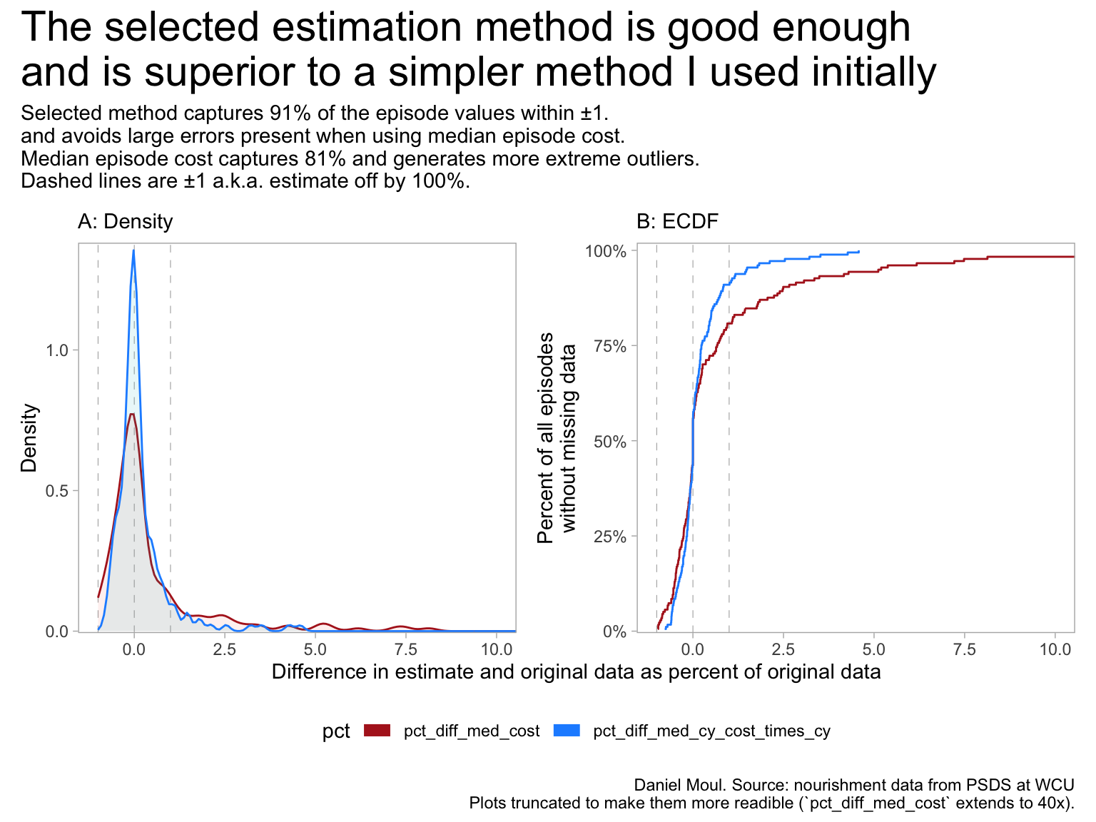
Where total cost and median cost are missing, volume_cy is typically available (and varies considerably among each place’s episodes). So using \(median(cost\_cy) * volume\_cy\) for each place (pct_diff_med_cy_cost_times_cy) is a better estimate than simply using \(median(cost)\) for each place (pct_diff_med_cost).
As an error check, the following plots compare the two estimation methods with the actual costs for those episodes that include costs (and thus in these cases I did not use estimated values in plots above). I assume the performance of the estimators is similar for episodes lacking cost data.
Show the code
dta_for_plot <- d_combined_with_est |>select(place, year_completed, adjusted_cost_2022, adjusted_cost_cy, med_adjusted_cost_2022, med_adjusted_cost_cy, adjusted_cost_2022_new) |>filter(!is.na(adjusted_cost_2022),!is.na(adjusted_cost_cy)) |>mutate(pct_diff_med_cost = (med_adjusted_cost_2022 - adjusted_cost_2022) / adjusted_cost_2022,pct_diff_med_cy_cost_times_cy = (adjusted_cost_2022_new - adjusted_cost_2022) / adjusted_cost_2022) |>pivot_longer(cols =contains("pct_diff"),names_to ="pct",values_to ="value")d_fun_a <- dta_for_plot |>filter(pct =="pct_diff_med_cy_cost_times_cy") |>pull(value) |>ecdf()prob_a <-d_fun_a(1) -d_fun_a(-1)d_fun_b <- dta_for_plot |>filter(pct =="pct_diff_med_cost") |>pull(value) |>ecdf()prob_b <-d_fun_b(1) -d_fun_b(-1)p1 <- dta_for_plot |>ggplot() +geom_vline(xintercept =c(-1, 0, 1), lty =2, linewidth =0.15, alpha =0.5) +geom_density(aes(value, color = pct, fill = pct),alpha =0.1,show.legend =FALSE) +scale_y_continuous(expand =expansion(mult =c(0.005, 0.02))) +scale_color_manual(values =c("firebrick", "dodgerblue")) +coord_cartesian(xlim =c(NA, 10)) +theme(legend.position ="bottom") +labs(subtitle ="A: Density",x ="Difference in estimate and original data as percent of original data",y ="Density" )p2 <- dta_for_plot|>ggplot() +geom_vline(xintercept =c(-1, 0, 1), lty =2, linewidth =0.15, alpha =0.5) +stat_ecdf(aes(value, color = pct),pad =FALSE,alpha =1) +scale_y_continuous(expand =expansion(mult =c(0.005, 0.02)),labels =label_percent()) +scale_color_manual(values =c("firebrick", "dodgerblue")) +guides(color =guide_legend(override.aes =list(linewidth =3))) +coord_cartesian(xlim =c(NA, 10)) +expand_limits(y =0) +theme(legend.position ="bottom") +labs(subtitle ="B: ECDF",x ="Difference in estimate and original data as percent of original data",y ="Percent of all episodes\nwithout missing data" )caption_extra2 <-glue("\nPlots truncated to make them more readible (`pct_diff_med_cost` extends to 40x).")p1 + p2 +plot_annotation(title =glue("The selected estimation method is good enough","\nand is superior to a simpler method I used initially"),subtitle =glue("Selected method captures {percent(prob_a)} of the episode values within ±1.", "\nand avoids large errors present when using median episode cost.","\nMedian episode cost captures {percent(prob_b)} and generates more extreme outliers.", "\nDashed lines are ±1 a.k.a. estimate off by 100%."),caption =paste0(my_caption, "\n", caption_extra2) ) +plot_layout(guides ="collect",axes ="collect") &theme(legend.position ="bottom")
Figure 1.15: The selected method of cost estimation is good enough
Note that I combined some locations in the source data as described in Section 2.4 Simplifying Categories.↩︎