The National Weather Service provides property damage estimates associated with tornadoes. The quality of the estimates limits what we can usefully do with it. As noted on the Storm Data FAQ Page:1
How are the damage amounts determined?
The National Weather Service makes a best guess using all available data at the time of the publication. The damage amounts are received from a variety of sources, including those listed above in the Data Sources section. Property and Crop damage should be considered as a broad estimate. Damage amounts are not adjusted for inflation and are the values that were entered at the time of the event.
Who surveys tornado damage? What’s the criteria for the National Weather Service to do a survey?
This varies from place to place; and there are no rigid criteria. The responsibility for damage survey decisions at each NWS office usually falls on the Warning-Coordination Meteorologist (WCM) and/or the Meteorologist in Charge (MIC). Budget constraints keep every tornado path from having a direct ground survey by NWS personnel; so spotter, chaser and news accounts may be used to rate relatively weak, remote or brief tornadoes. Killer tornadoes, those striking densely populated areas, or those generating reports of exceptional damage are given highest priority for ground surveys. Most ground surveys involve the WCM and/or forecasters not having shift responsibility the day of the survey. For outbreaks and unusually destructive events–usually only a few times a year–the NWS may support involvement by highly experienced damage survey experts and wind engineers from elsewhere in the country. Aerial surveys are expensive and usually reserved for tornado events with multiple casualties and/or massive degrees of damage. Sometimes, local NWS offices may have a cooperative agreement with local media, law enforcement, or Civil Air Patrol to use their aircraft during surveys. Unmanned aerial vehicles (drones) also can be used to map and find tornado damage, but are not always available.
There are also data entry errors. For example, the record of the Beaufort County tornado on April 25, 2014 (Table 1 event 505635) includes estimated property damage of $1.5 million while the NWS’s narrative states $15 million. In this case I adjusted the estimated property damage value.
2.1 Most property damage
Show the code
ggplot() +geom_sf(data = nc_counties,fill =NA, linewidth =0.05) +geom_sf(data = nc_cities,fill ="grey85", color =NA) +geom_sf(data = nc_state,fill =NA, linewidth =0.5,color ="grey") +geom_sf(data = dta |>slice_max(damage_property_mil_2022, n =10),aes(color = damage_property_mil_2022)) +#scale_color_continuous(trans = "log2") +scale_color_gradient2(low =muted("blue"),high =muted("red"),trans ="log2") +# scale_color_viridis_c(end = 0.85,# trans = "log2") +theme(panel.background =element_blank(),panel.border =element_blank(),panel.grid =element_blank(),axis.text =element_blank(),axis.ticks =element_blank(),plot.title =element_text(size =rel(2.0), face ="bold"),legend.position =c(0.3, 0.3)) +labs(title =glue("Top tornadoes causing ten largest amounts of estimated property damage", "\nin North Carolina 1970-01-01 to 2023-04-30"),subtitle ="In millions of 2022 dollars",caption = my_caption )
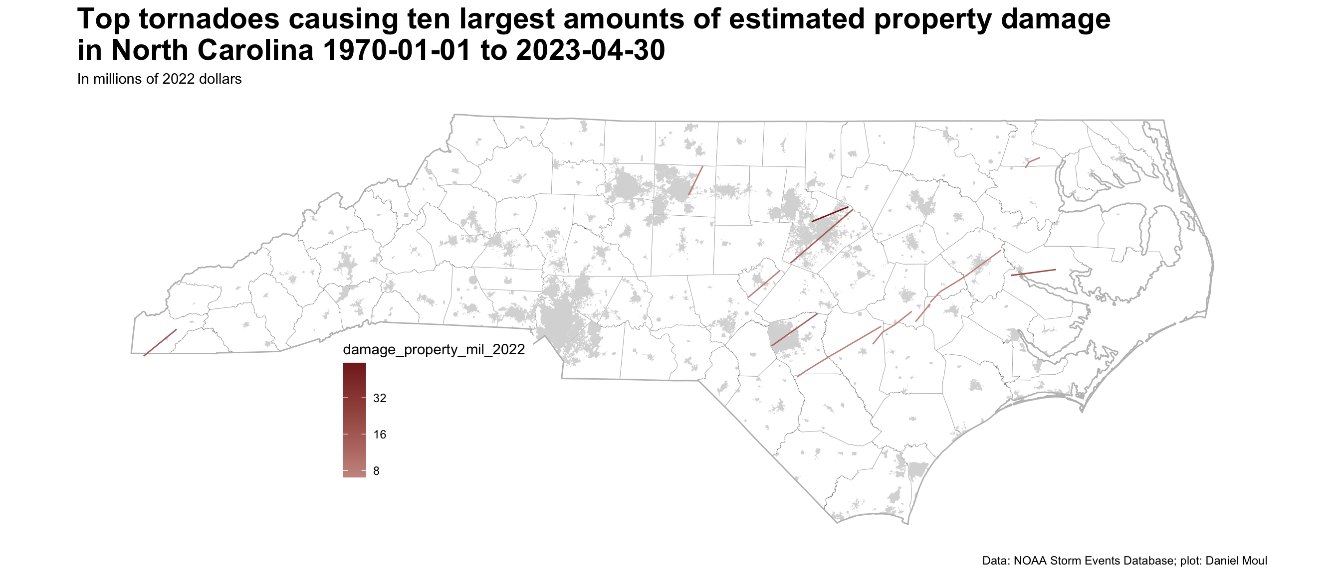
Figure 2.1: Top tornadoes causing ten largest amounts of estimated property damage in NC 1970-01-01 to 2023-04-30.
Show the code
data_for_modeling_with_cities |>st_drop_geometry() |>slice_max(damage_property_mil_2022, n =10) |>select(damage_property_mil_2022, n_intersects, length_mi, year, tor_f_scale, injuries_direct, injuries_indirect, deaths_direct, deaths_indirect) |>mutate(length_mi =drop_units(length_mi)) |>arrange(desc(damage_property_mil_2022)) |>gt() |>tab_header(md(glue("**Top tornadoes causing ten largest amounts of estimated property damage in NC since {year_start}**"))) |>fmt_number(columns = damage_property_mil_2022,decimals =3) |>fmt_number(columns = length_mi,decimals =1) |>tab_source_note(md("*Data: NOAA Storm Events Database; analysis: Daniel Moul<br>damage_property_mil in millions of 2022 dollars*"))
Top tornadoes causing ten largest amounts of estimated property damage in NC since 1971
damage_property_mil_2022
n_intersects
length_mi
year
tor_f_scale
injuries_direct
injuries_indirect
deaths_direct
deaths_indirect
61.855
2
18.2
1988
4
105
0
2
0
18.549
1
21.0
2014
3
16
0
0
1
14.967
4
38.0
2011
3
67
0
4
0
14.843
1
19.7
1974
4
26
0
4
0
13.015
1
26.2
2011
3
85
0
1
0
8.979
1
0.0
1998
3
5
0
0
0
7.577
1
15.1
2018
2
0
2
0
1
7.418
1
19.1
2011
3
36
0
2
0
7.043
0
4.8
1984
3
0
0
0
0
7.043
0
13.3
1984
3
11
0
2
0
7.043
0
27.5
1984
3
90
0
10
0
7.043
0
7.1
1984
4
50
0
0
0
7.043
0
6.6
1984
4
40
0
0
0
7.043
0
6.2
1984
3
74
0
0
0
7.043
1
4.5
1984
3
7
0
0
0
7.043
1
10.1
1984
4
59
0
3
0
7.043
0
6.6
1984
4
0
0
0
0
7.043
0
13.2
1984
4
0
0
7
0
7.043
1
3.2
1984
2
2
0
0
0
7.043
1
5.4
1984
2
5
0
0
0
7.043
2
21.0
1984
4
153
0
9
0
Data: NOAA Storm Events Database; analysis: Daniel Moul damage_property_mil in millions of 2022 dollars
Show the code
data_for_modeling_with_cities |>st_drop_geometry() |>slice_max(length_mi, n =10) |>select(length_mi, damage_property_mil, n_intersects, year, tor_f_scale, injuries_direct, injuries_indirect, deaths_direct, deaths_indirect) |>mutate(length_mi =drop_units(length_mi)) |>arrange(desc(damage_property_mil)) |>gt() |>tab_header(md(glue("**Ten longest tornadoes tracks and related property damage in NC since {year_start}**"))) |>fmt_number(columns = damage_property_mil,decimals =3) |>fmt_number(columns = length_mi,decimals =1) |>tab_source_note(md("*Data: NOAA Storm Events Database; analysis: Daniel Moul<br>damage_property_mil in millions of dollars; not adjusted for inflation*"))
Ten longest tornadoes tracks and related property damage in NC since 1971
length_mi
damage_property_mil
n_intersects
year
tor_f_scale
injuries_direct
injuries_indirect
deaths_direct
deaths_indirect
38.0
11.500
4
2011
3
67
0
4
0
30.3
0.250
2
1992
3
12
0
0
0
29.0
0.250
2
1991
2
0
0
0
0
28.1
0.250
1
1984
4
280
0
2
0
64.0
0.025
2
1971
1
0
0
0
0
44.2
0.025
1
1971
2
0
0
0
0
31.6
0.025
0
1992
3
0
0
0
0
31.5
0.025
4
1973
1
0
0
0
0
30.9
0.025
2
1975
2
1
0
0
0
69.6
0.000
1
1971
3
0
0
0
0
Data: NOAA Storm Events Database; analysis: Daniel Moul damage_property_mil in millions of dollars; not adjusted for inflation
2.2 Variable associations with property damage
The models below explain between 10% and 15% of the variance–a surprisingly low amount. I’m using nominal dollars (not adjusted for inflation), since the model results are a little better than when using constant dollars.
In the models above, if a term changes by \(1\), it results in an estimate change in the property damage in millions of dollars (nominial dollars–not adjusted for inflation).
Adjusted \(R^2\) is the proportion of the variance explained by the linear regression.
mod1: there is not much correlation between property damage and force of the tornado.
mod2: there is not much correlation between property damage and the length of the tornado track.
mod3: there is not much correlation between property damage and both force and length of track.
mod4:including the number of intersections with populated areas does not improve the model materially. This is a surprise, since it seems to me the property damage would be higher the more times the tornado passes over a populated area.
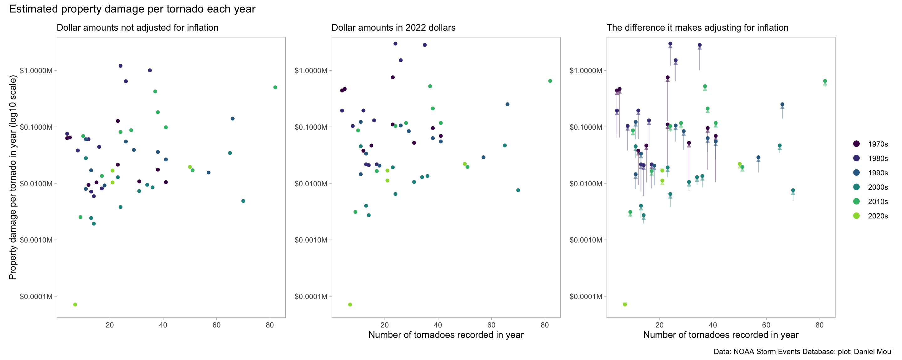
2.3 Property damage per year
First a short digression: nominal dollars (not adjusted for inflation) over 50 years paints a distorted picture. Figure 2.2 presents the difference in perspective.
Show the code
yearly_property_damage <- dta_non_mapping |>st_drop_geometry() |>reframe(damage_property_mil =sum(damage_property_mil),damage_property_mil_2022 =sum(damage_property_mil_2022),n_tornadoes =n(),.by = year) |>mutate(damage_prop_mil_per_tornado = damage_property_mil / n_tornadoes,damage_prop_mil_2022_per_tornado = damage_property_mil_2022 / n_tornadoes,decade =as.factor(paste0(floor(year /10) *10, "s")))scale_y_max <-max(yearly_property_damage$damage_prop_mil_2022_per_tornado, na.rm =TRUE)scale_y_min <-min(yearly_property_damage$damage_prop_mil_2022_per_tornado, na.rm =TRUE)p1 <- yearly_property_damage |>ggplot(aes(n_tornadoes, damage_prop_mil_per_tornado, color = decade)) +geom_point(show.legend =FALSE) +scale_x_continuous() +#expand = expansion(mult = c(0.01, 0.02))) +scale_y_log10(labels =label_number(prefix ="$", suffix ="M"),expand =expansion(mult =c(0.01, 0.02))) +scale_color_viridis_d(end =0.85) +coord_cartesian(ylim =c(0.65* scale_y_min, 1.05* scale_y_max)) +theme(panel.grid =element_blank(),plot.title =element_text(size =rel(2.0), face ="bold"),legend.position ="right") +guides(color =guide_legend(override.aes =list(size =3))) +labs(subtitle ="Dollar amounts not adjusted for inflation",x =NULL,x ="Number of tornadoes recorded in year",y ="Property damage per tornado in year (log10 scale)",color =NULL, )p2 <- yearly_property_damage |>ggplot(aes(n_tornadoes, damage_prop_mil_2022_per_tornado, color = decade)) +geom_point(show.legend =FALSE) +scale_x_continuous() +#expand = expansion(mult = c(0.01, 0.02))) +scale_y_log10(labels =label_number(prefix ="$", suffix ="M"),expand =expansion(mult =c(0.01, 0.02))) +scale_color_viridis_d(end =0.85) +coord_cartesian(ylim =c(0.65* scale_y_min, 1.05* scale_y_max)) +theme(panel.grid =element_blank(),plot.title =element_text(size =rel(2.0), face ="bold"),legend.position ="right") +guides(color =guide_legend(override.aes =list(size =3))) +labs(subtitle ="Dollar amounts in 2022 dollars",x ="Number of tornadoes recorded in year",y =NULL,color =NULL, )p3 <- yearly_property_damage |>ggplot() +geom_segment(aes(x = n_tornadoes, xend = n_tornadoes, y = damage_prop_mil_per_tornado, yend =0.95* damage_prop_mil_2022_per_tornado, color = decade), linewidth =0.4, alpha =0.4,arrow =arrow(length =unit(1.5, "mm"),ends ="last",type ="closed"),show.legend =FALSE) +#geom_point(aes(x = n_tornadoes, y = damage_prop_mil_per_tornado, color = decade)) + geom_point(aes(x = n_tornadoes, y = damage_prop_mil_2022_per_tornado, color = decade)) +scale_x_continuous() +#expand = expansion(mult = c(0.01, 0.02))) +scale_y_log10(labels =label_number(prefix ="$", suffix ="M"),expand =expansion(mult =c(0.01, 0.02))) +scale_color_viridis_d(end =0.85) +coord_cartesian(ylim =c(0.65* scale_y_min, 1.05* scale_y_max)) +theme(panel.grid =element_blank(),plot.title =element_text(size =rel(2.0), face ="bold"),legend.position ="right") +guides(color =guide_legend(override.aes =list(size =3,linewidth =0))) +labs(subtitle ="The difference it makes adjusting for inflation",x ="Number of tornadoes recorded in year",y =NULL,color =NULL, )p1 + p2 + p3 +plot_annotation(title ="Estimated property damage per tornado each year",caption = my_caption )
Figure 2.2: Property damage per tornado yearly
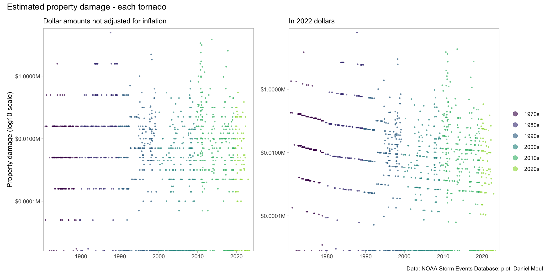
Before about 1996 it seems there were standard values used for property damage estimates, and even since then some values seem too common to be more than often-used estimates.
yearly_property_damage |>select(-decade) |>gt() |>tab_header(md(glue("**Estimated yearly property damage in NC caused by tornadoes**", "<br>January 1, {year_start} to April 30, 2023"))) |>fmt_number(columns =c(damage_property_mil, damage_property_mil_2022, damage_prop_mil_per_tornado, damage_prop_mil_2022_per_tornado),decimals =3) |>tab_source_note(md("*Data: NOAA Storm Events Database; analysis: Daniel Moul<br>damage_property_mil in millions of dollars*"))
Estimated yearly property damage in NC caused by tornadoes January 1, 1971 to April 30, 2023
year
damage_property_mil
damage_property_mil_2022
n_tornadoes
damage_prop_mil_per_tornado
damage_prop_mil_2022_per_tornado
1971
0.325
2.349
5
0.065
0.470
1972
0.253
1.768
4
0.063
0.442
1973
0.431
2.838
41
0.011
0.069
1974
2.928
17.385
23
0.127
0.756
1975
0.666
3.622
38
0.018
0.095
1976
0.494
2.540
23
0.021
0.110
1977
0.336
1.622
31
0.011
0.052
1978
0.156
0.702
15
0.010
0.047
1979
0.113
0.454
12
0.009
0.038
1980
0.083
0.294
14
0.006
0.021
1981
0.728
2.343
12
0.061
0.195
1982
0.093
0.282
13
0.007
0.022
1983
0.710
2.087
16
0.044
0.130
1984
35.160
99.051
35
1.005
2.830
1985
0.306
0.832
8
0.038
0.104
1986
0.138
0.369
17
0.008
0.022
1987
0.302
0.779
4
0.076
0.195
1988
29.006
71.766
24
1.209
2.990
1989
16.710
39.444
26
0.643
1.517
1990
0.166
0.371
18
0.009
0.021
1991
1.136
2.442
29
0.039
0.084
1992
1.087
2.267
41
0.027
0.055
1993
0.666
1.349
11
0.061
0.123
1994
0.222
0.437
13
0.017
0.034
1995
1.434
2.754
26
0.055
0.106
1996
0.887
1.654
57
0.016
0.029
1997
0.088
0.160
11
0.008
0.015
1998
9.269
16.644
66
0.140
0.252
1999
1.367
2.402
38
0.036
0.063
2000
0.092
0.156
24
0.004
0.006
2001
0.032
0.052
13
0.002
0.004
2002
0.307
0.500
11
0.028
0.045
2003
0.306
0.486
36
0.008
0.014
2004
0.342
0.530
70
0.005
0.008
2005
0.295
0.442
23
0.013
0.019
2006
0.227
0.329
31
0.007
0.011
2007
0.027
0.038
14
0.002
0.003
2008
2.246
3.053
65
0.035
0.047
2009
0.321
0.438
34
0.009
0.013
2010
2.449
3.286
28
0.087
0.117
2011
41.165
53.575
82
0.502
0.653
2012
1.955
2.492
24
0.081
0.104
2013
0.690
0.867
10
0.069
0.087
2014
15.745
19.471
37
0.426
0.526
2015
0.023
0.028
9
0.003
0.003
2016
0.231
0.281
17
0.014
0.017
2017
4.033
4.817
41
0.098
0.117
2018
6.916
8.062
38
0.182
0.212
2019
0.870
0.996
51
0.017
0.020
2020
0.980
1.108
50
0.020
0.022
2021
0.218
0.236
21
0.010
0.011
2022
0.354
0.354
21
0.017
0.017
2023
0.001
0.001
7
0.000
0.000
Data: NOAA Storm Events Database; analysis: Daniel Moul damage_property_mil in millions of dollars