2  Voyage maps

Show the code
source(here::here("scripts/setup.R"))

# World map example from https://www.simoncoulombe.com/2020/11/animated-ships/
  
world <- rnaturalearth::ne_countries(scale='medium',returnclass = 'sf') %>%
  st_transform(crs = my_proj)

# create water polygon for background 
lats <- c(90:-90, -90:90, 90)
longs <- c(rep(c(180, -180), each = 181), 180)
water_outline <- 
  list(cbind(longs, lats)) %>%
  st_polygon() %>%
  st_sfc(crs = "+proj=longlat +ellps=WGS84 +datum=WGS84 +no_defs") %>% 
  st_sf() %>%
  st_transform(crs = my_proj)

source(here("scripts/load-voyages.R"))

source(here("scripts/plot-voyages-functions.R"))

2.1 Maps: North America

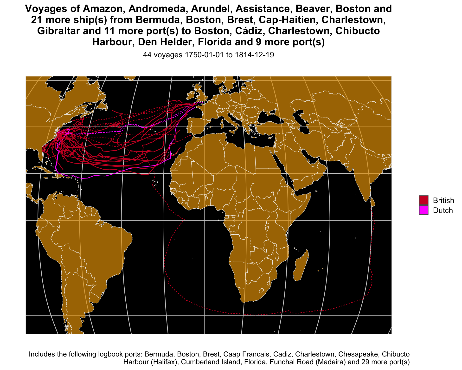
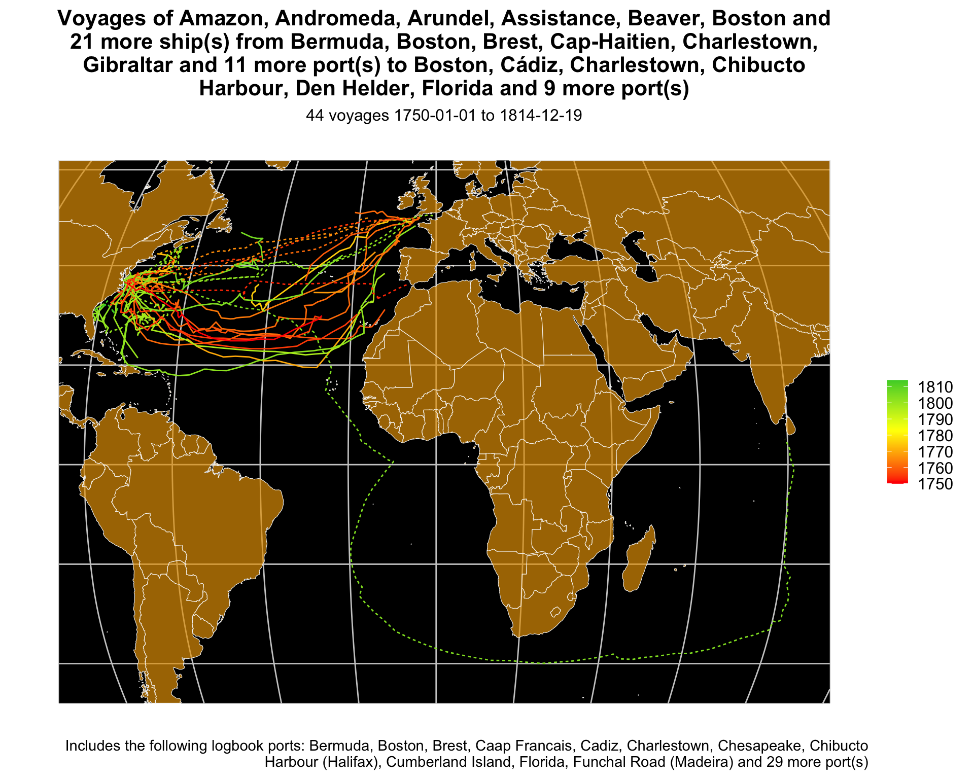
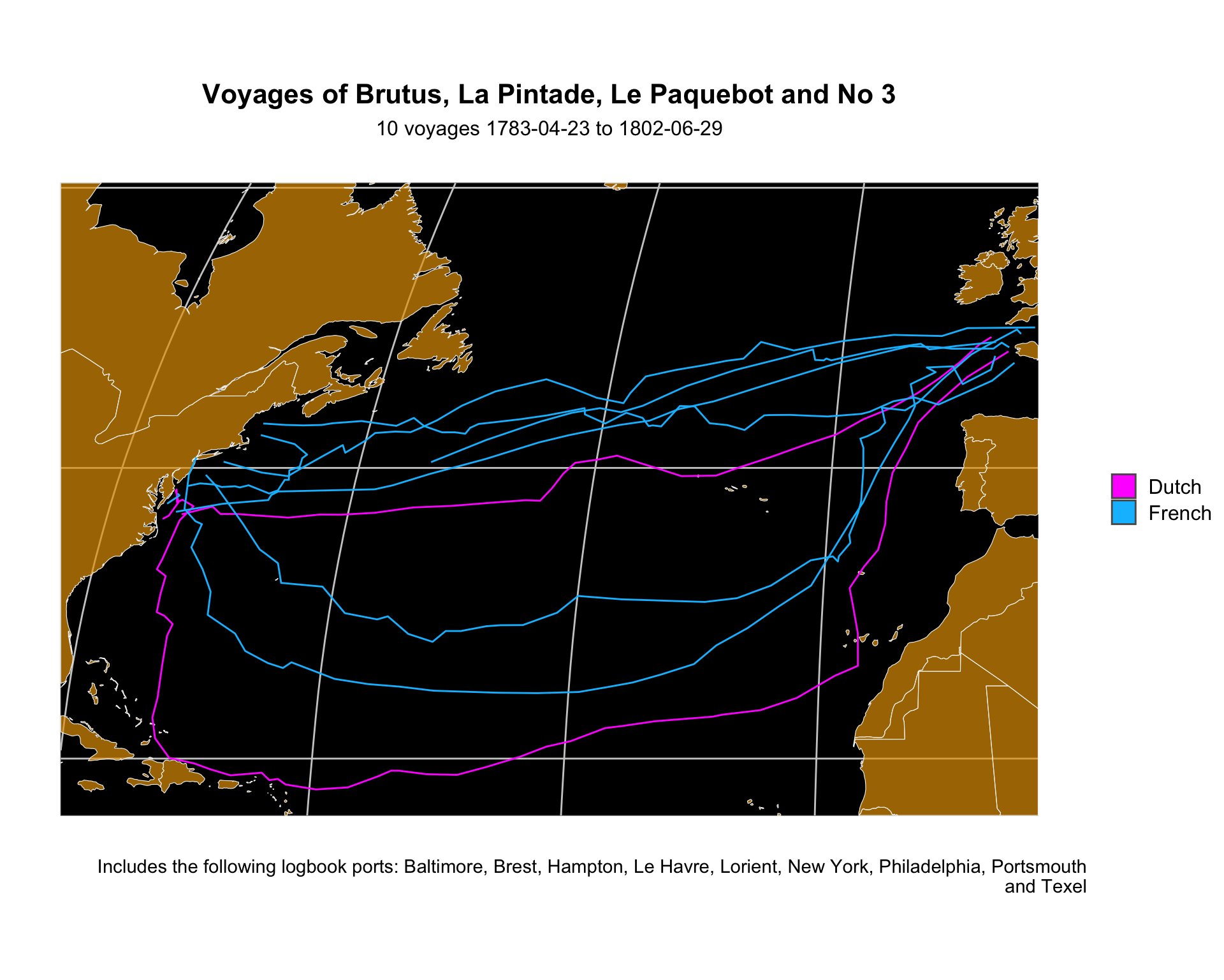
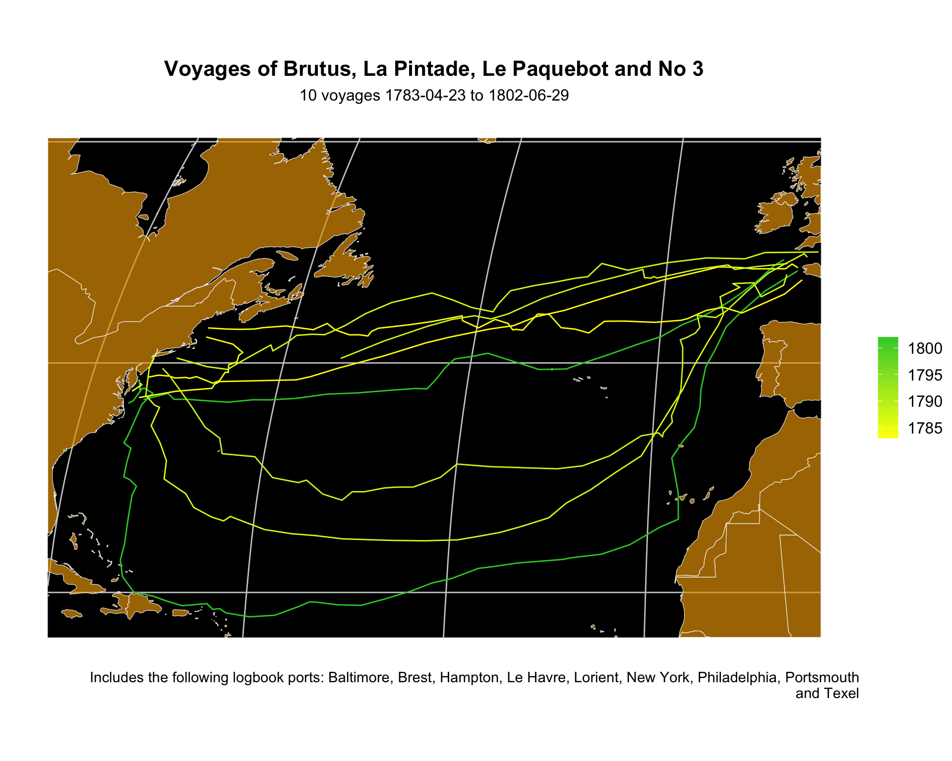
2.1.1 Voyages to or from Virginia (“Hampton Road”)

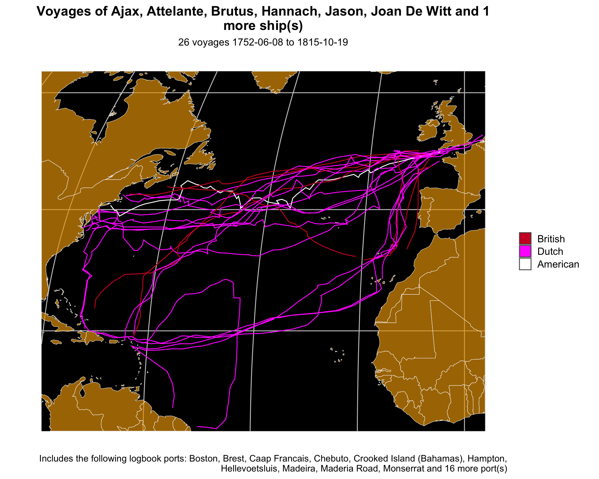
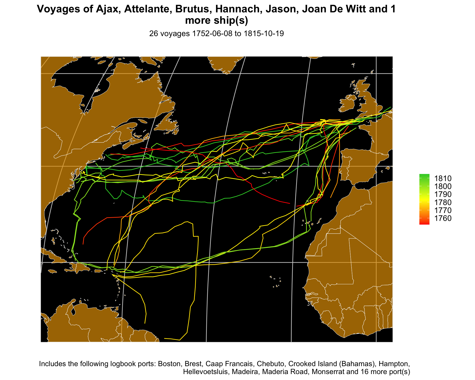
British ships made most of the voyages to Virginia in this data set; Dutch ships made a few. We see a pattern in the routes between the Mid-Atlantic coast and Northern Europe, due to the prevailing winds: when leaving Europe, south near the Azores or Canary Islands then west across the Atlantic; when leaving North America: a more northerly path.

See also table Section 3.1.

Show the code
voyage_list <- df_voyages %>% 
               filter(port_from == "hampton road" | port_to == "hampton road")

plot_voyages(ships = voyage_list$ShipName,
             from = "hampton road",
             to = "hampton road"
)
Figure 2.1: Voyages to or from Hampton Roads, Virginia


Looking at the same voyages by year, we see nearly the whole time period represented.

Show the code
plot_voyages(ships = voyage_list$ShipName,
             from = "hampton road",
             to = "hampton road",
             color_var = "year"
)
Figure 2.2: Voyages to or from Hampton Roads, Virginia, by year


2.1.2 Voyages between US and lands

Our data set includes Dutch voyages from Boston, New York, and Virginia. All occurred after US independence–the first one directly after.

See also table Section 3.2.

Show the code
ship_list <- 
  c(df_voyages %>% 
      filter(country_from == "united states" & country_to == "netherlands") %>%
      pull(ShipName),
    df_voyages %>%
      filter(country_from == "netherlands" & country_to == "united states") %>%
      pull(ShipName)
  )

plot_voyages(ships = ship_list)
plot_voyages(ships = ship_list,
             color_var = "year")
Figure 2.3: Voyages between the U.S. and Netherlands
Figure 2.4: Voyages between the U.S. and Netherlands


2.1.3 Voyages between US and France

These voyages occurred in the final months of the American Revolutionary War in 1783 and afterwards.

Show the code
ship_list <- 
  c(df_voyages %>% 
      filter(country_from == "united states" & country_to == "france") %>%
      pull(ShipName),
    df_voyages %>%
      filter(country_from == "france" & country_to == "united states") %>%
      pull(ShipName)
  )

plot_voyages(ships = ship_list)

plot_voyages(ships = ship_list,
             color_var = "year")
Figure 2.5: Voyages between the U.S. and France
Figure 2.6: Voyages between the U.S. and France


2.1.4 Voyages between Canada and France

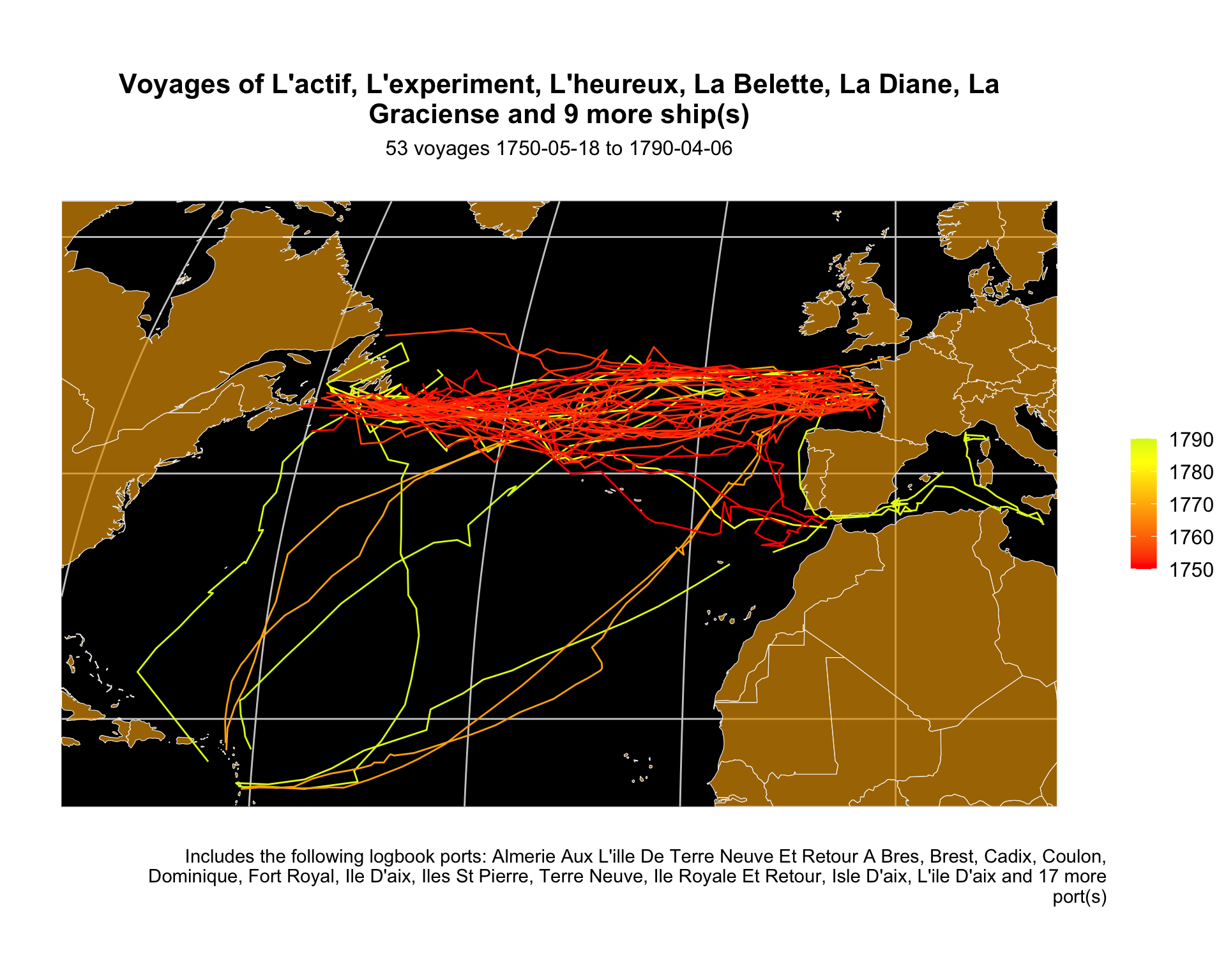
Most French voyages occurred before or during the Seven Years War, after which France’s territorial holdings in North America were limited to the small islands of St Pierre and Miquelon. They remain a part of France today.

See also table Section 3.3.

Show the code
ship_list <- 
  c(df_voyages %>% 
      filter(country_from == "canada" & country_to == "france") %>%
      pull(ShipName),
    df_voyages %>%
      filter(country_from == "france" & country_to == "canada") %>%
      pull(ShipName)
  )

plot_voyages(ships = ship_list,
             color_var = "year")
Figure 2.7: Voyages between Canada and France


2.1.5 Voyages to or from Florida

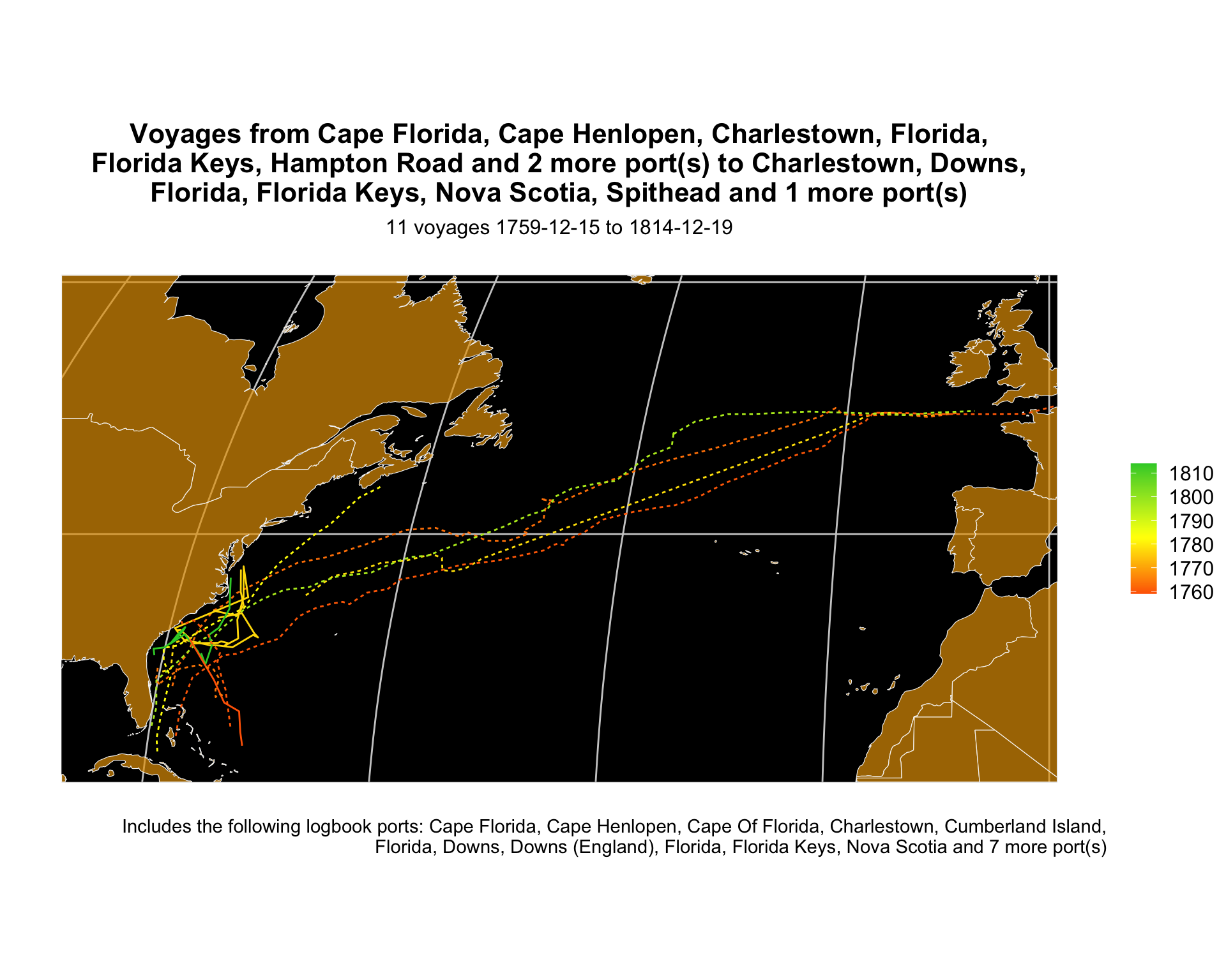
St. Augustine was founded in 1565 by Spanish explorers and has been inhabited continuously since then–the longest of any city in the continental US. It became the capital of British East Florida in 1763, returned to Spanish control in 1783, then Spain ceded it to the USA in 1819. Our data set includes only British voyages.

See also table Section 3.4.

Show the code
plot_voyages(
  from = filter(df_ports, level2 == "florida") %>% pull(port2),
  to = filter(df_ports, level2 == "florida") %>% pull(port2),
  color_var = "year"
)
Figure 2.8: Voyages to or from Florida


2.1.6 All voyages of ships that went to to or from Florida at least once

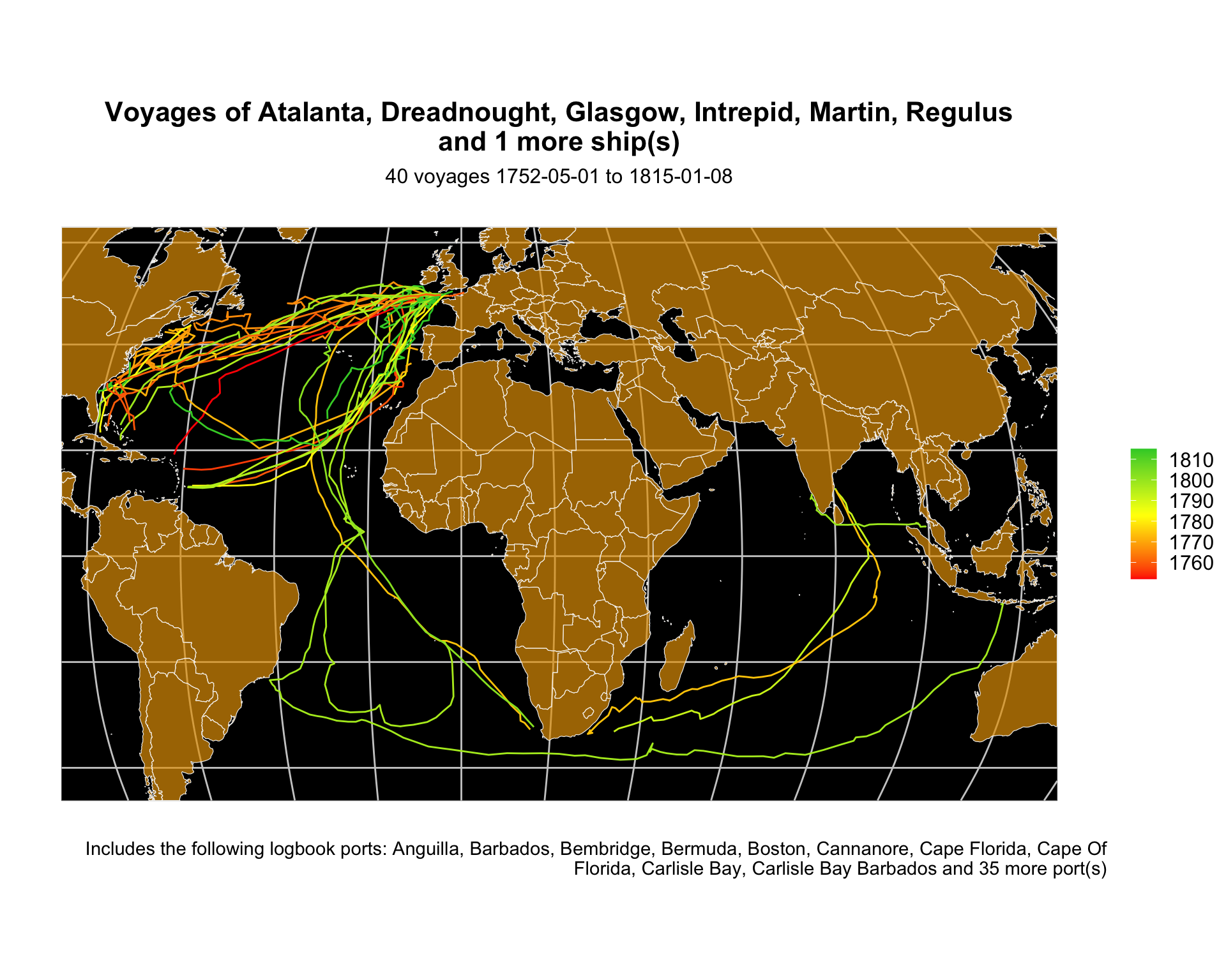
Looking at all the voyages in our data set undertaken by ships that traveled from or to Florida, we see a much wider web going as far as India, Ceylon (now Sri Lanka), Malaysia, and the Dutch East Indies (now Indonesia and nearby island nations). These 27 ships were part of the British Royal Navy.

Show the code
voyage_list <- df_voyages %>% 
               filter(str_detect(port_to, "florida") | str_detect(port_from, "florida"))

plot_voyages(ships = voyage_list$ShipName,
             color_var = "year")
Figure 2.9: All voyages of ships that went to or from Florida at least once


2.1.7 Voyages to or from Veracruz, Mexico

The primary port in the Spanish colony of Mexico was Veracruz. Cuba was settled earlier and remained a regional center in this time period.

Show the code
plot_voyages(to = "veracruz")
plot_voyages(to = "veracruz", color_var = "year")
plot_voyages(from = "veracruz")
plot_voyages(from = "veracruz", color_var = "year")
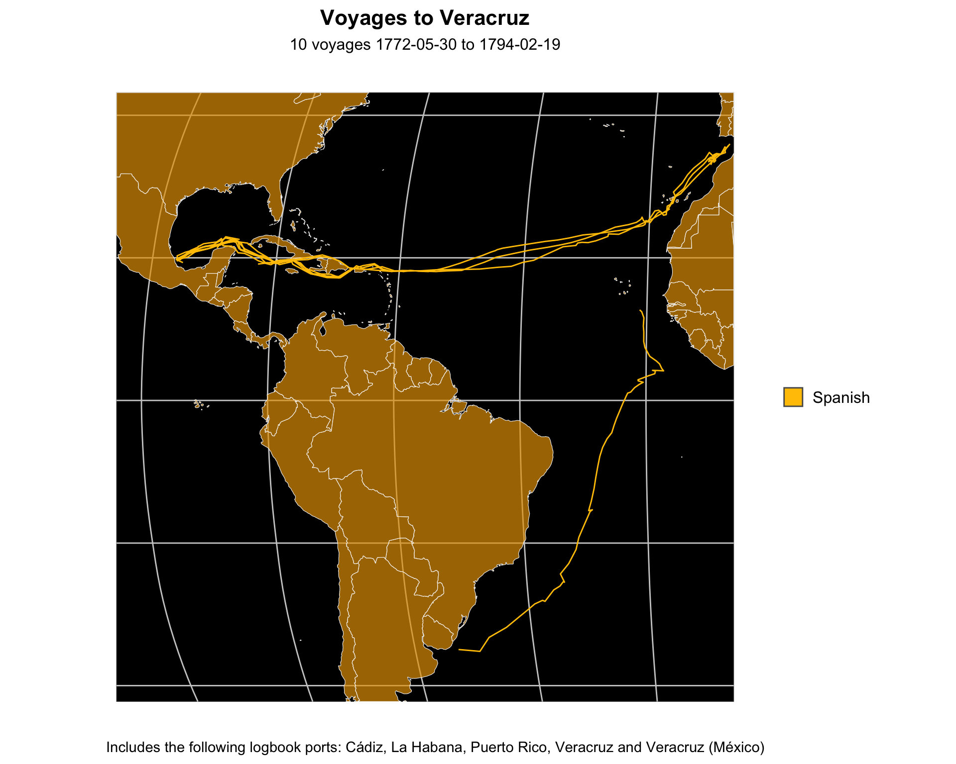
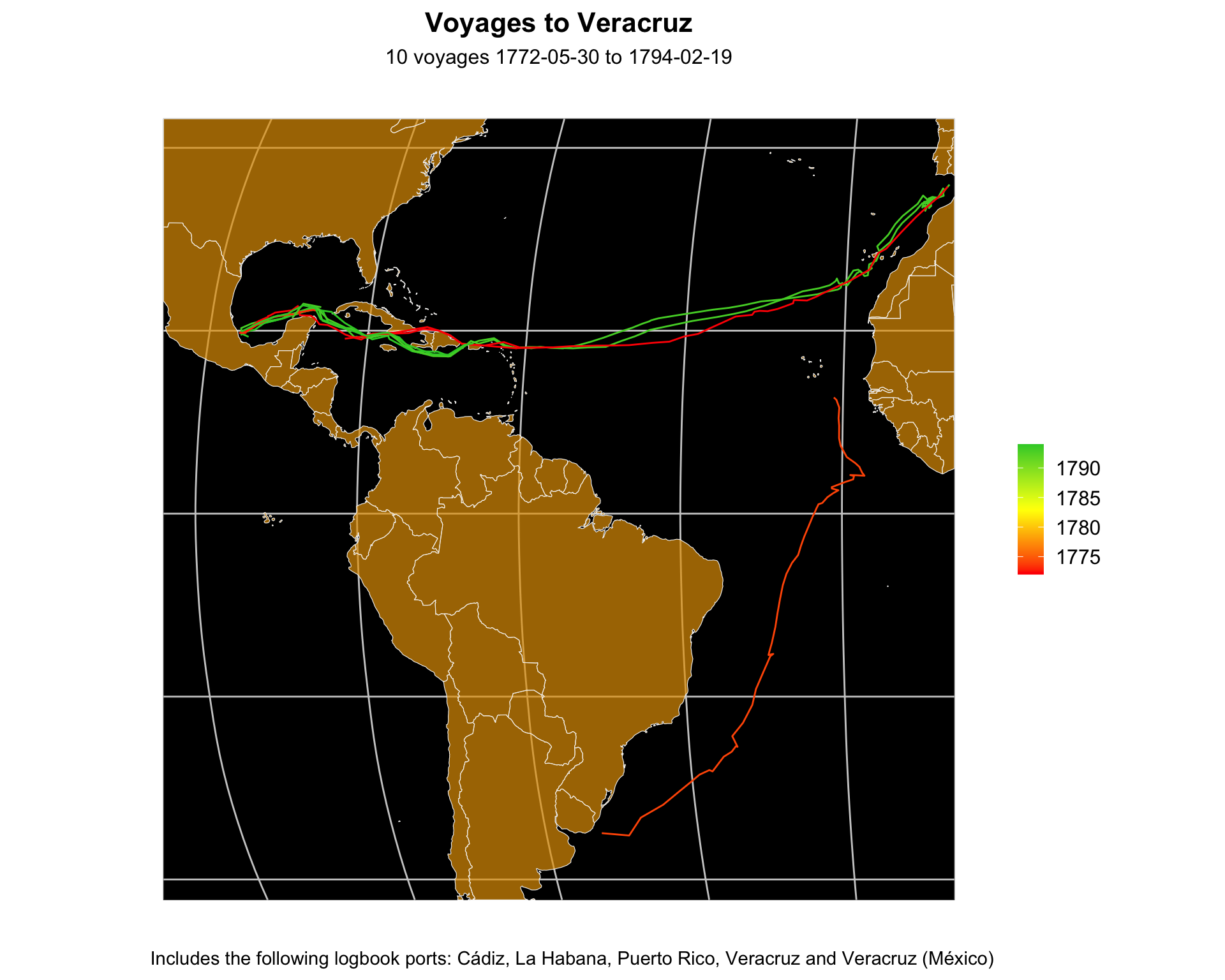
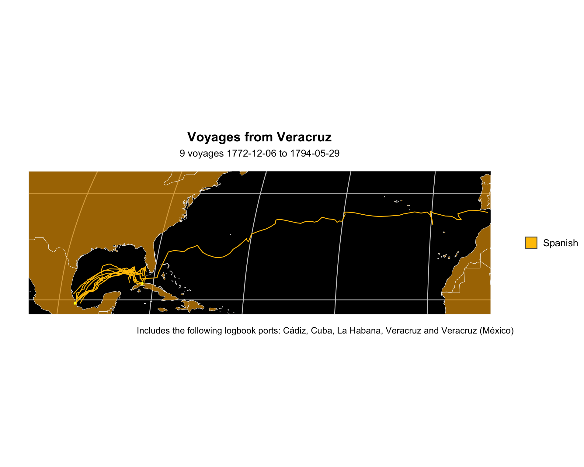
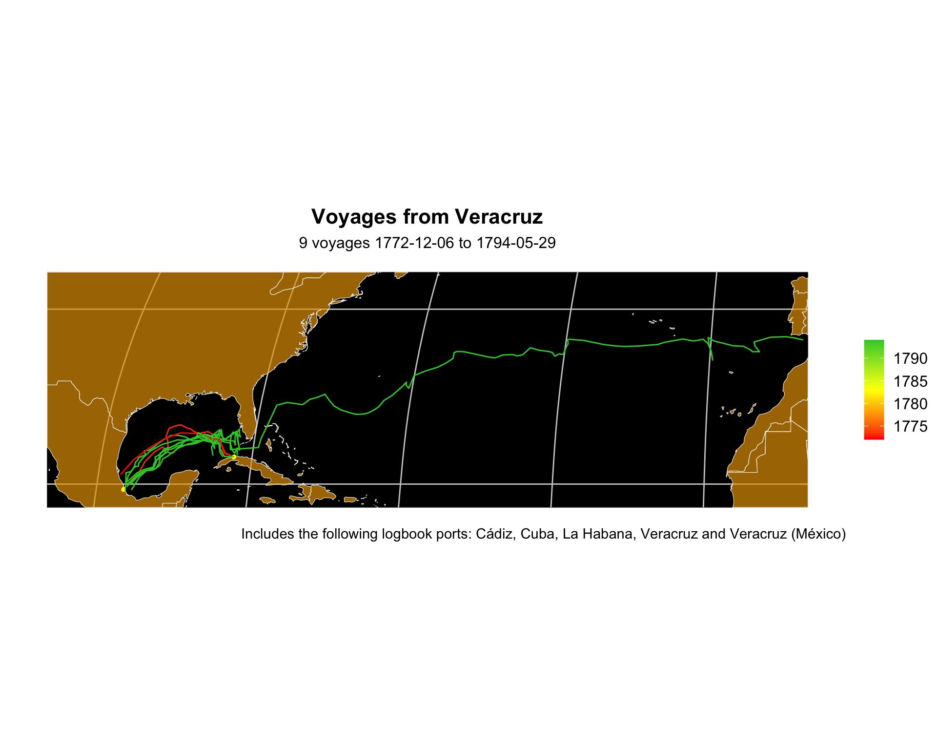
Figure 2.10: All voyages to or from Veracruz, Mexico
Figure 2.11: All voyages to or from Veracruz, Mexico
Figure 2.12: All voyages to or from Veracruz, Mexico
Figure 2.13: All voyages to or from Veracruz, Mexico

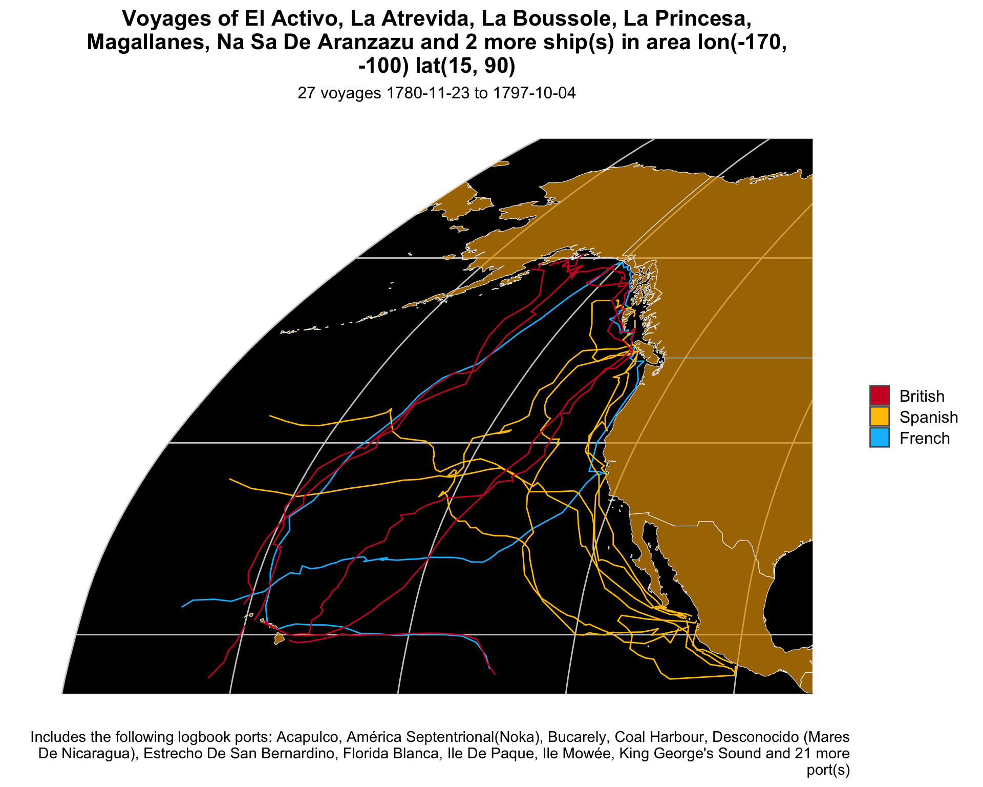
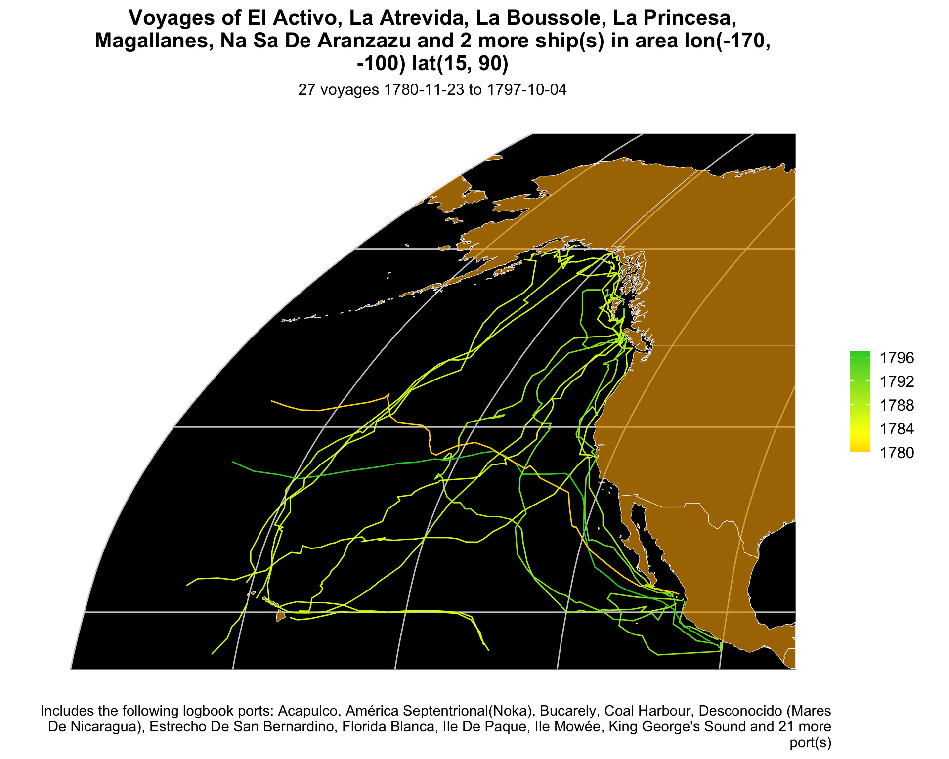
2.1.8 Explorations of the northwest coast of North America

Our data set includes Spanish, British and French voyages of discovery along the western coast of North America. The Spanish went further south; the British, further north.

See also table Section 3.4.1.

Show the code
nw_explorers <- 
  get_voyage_details(range_lon = c(-170, -100),
                     range_lat = c(15, 90)
                     )

plot_voyages(ships = nw_explorers$ShipName,
             range_lon = c(-170, -100),
             range_lat = c(15, 90)
)

plot_voyages(ships = nw_explorers$ShipName,
             range_lon = c(-170, -100),
             range_lat = c(15, 90),
             color_var = "year")
Figure 2.14: All voyages to or from the US Coastal Northwest
Figure 2.15: All voyages to or from the US Coastal Northwest


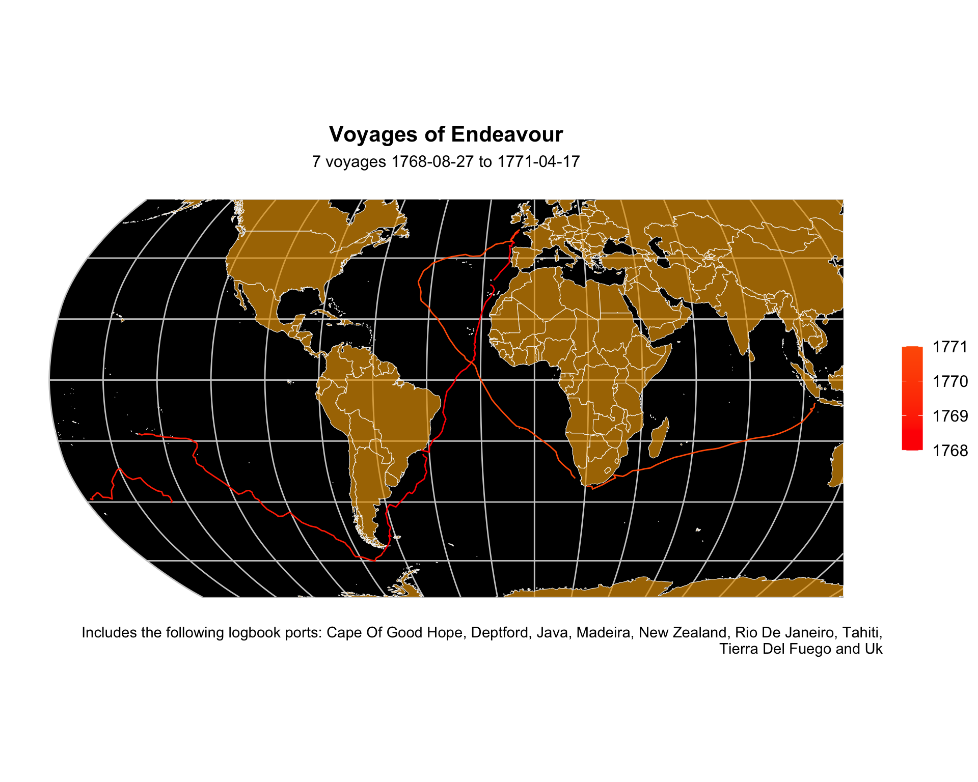
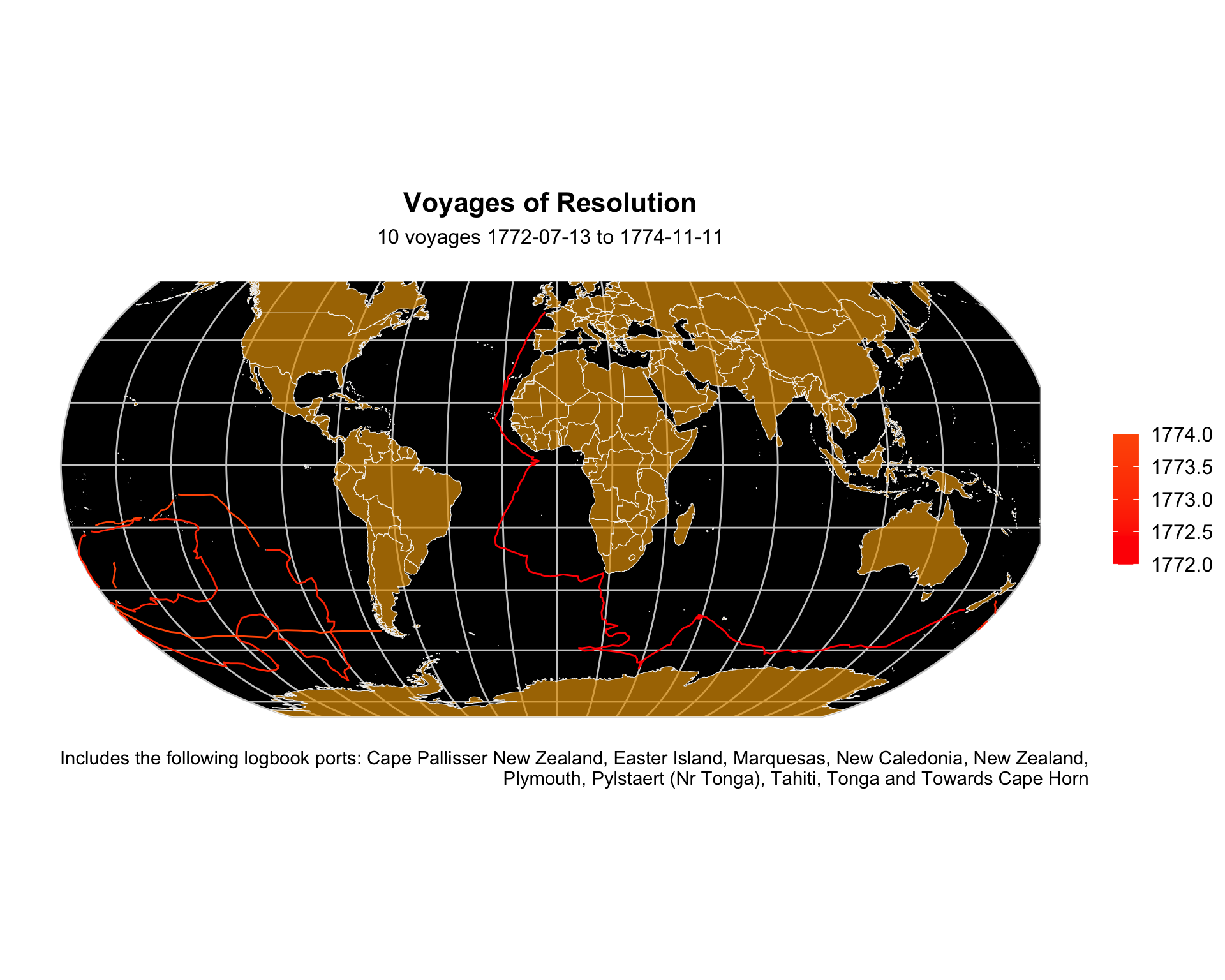
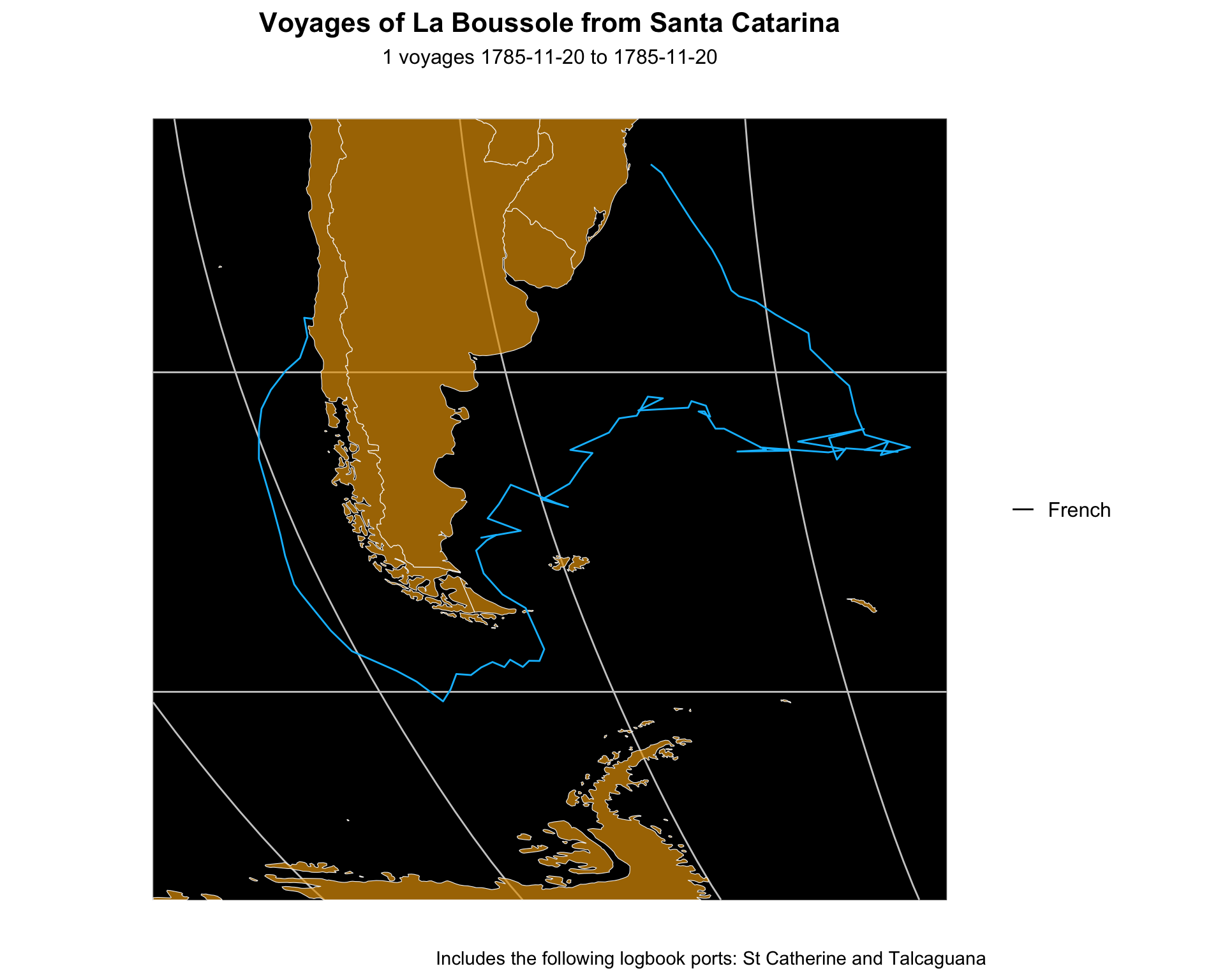
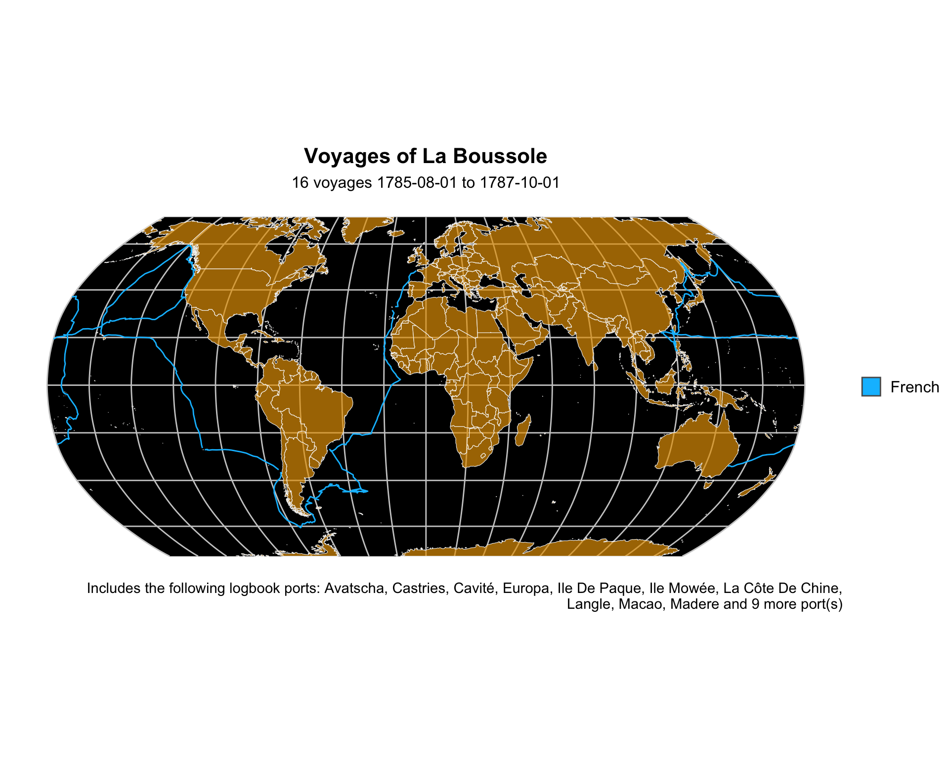
2.2 James Cook’s first and second voyages of discovery

Our data set includes portions of James Cook’s first circumnavigation westward for the purpose of observing the 1769 transit of Venus in Tahiti and then searching for unknown land to the south, Terra Astralis, Incognita, believed to exist further south than Australia, which was then called New Holland. On this journey he landed in Australia at a place he named Botany Bay in present-day Sydney. Our records include portions of Cook’s second oyage from Britain eastward to New Zealand and eventually around the South American cape and back to Britain. He never found Antarctica, despite coming close, and his experience convinced people that Terra Astralis Incognita did not exist.

See also table Section 3.5.

Show the code
ship_list <- c("ENDEAVOUR", "RESOLUTION")
cooks_first_journey <- c("1768-01-01", "1771-12-31")
cooks_second_journey <- c("1772-01-01", "1775-12-31")

plot_voyages(ships = ship_list,
             range_dates = cooks_first_journey,
             color_var = "year"
)

plot_voyages(ships = ship_list,
             range_dates = cooks_second_journey,
             color_var = "year"
)
Figure 2.16: James Cook’s voyages in the data set
Figure 2.17: James Cook’s voyages in the data set

2.3 Maps: South America

2.3.1 To and or from Brazil, Uruguay, Argentina

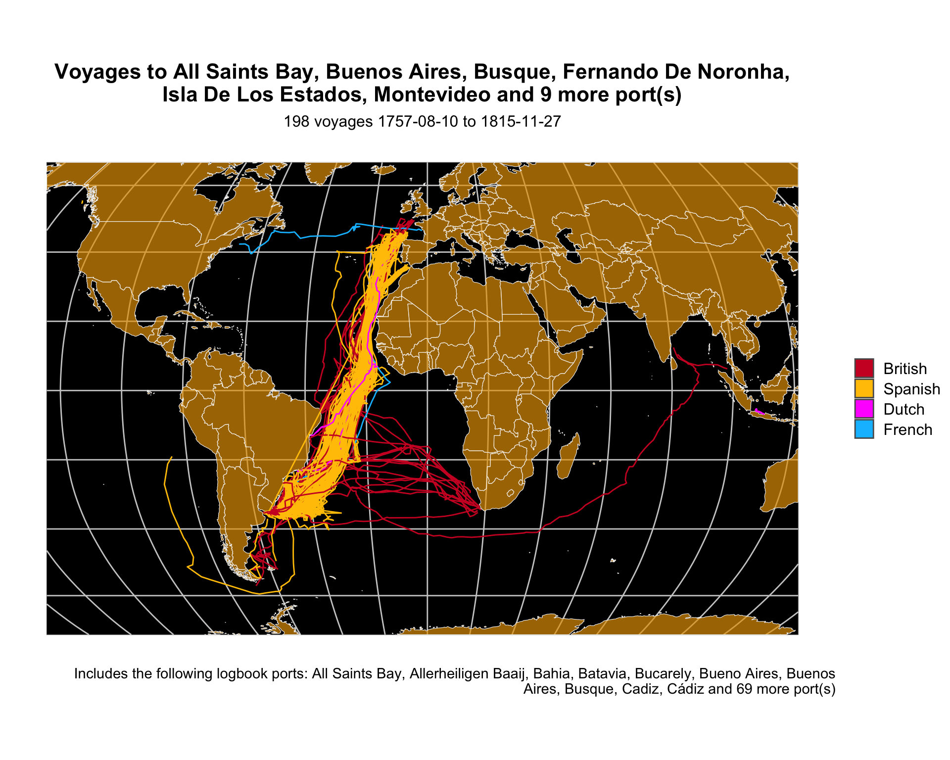
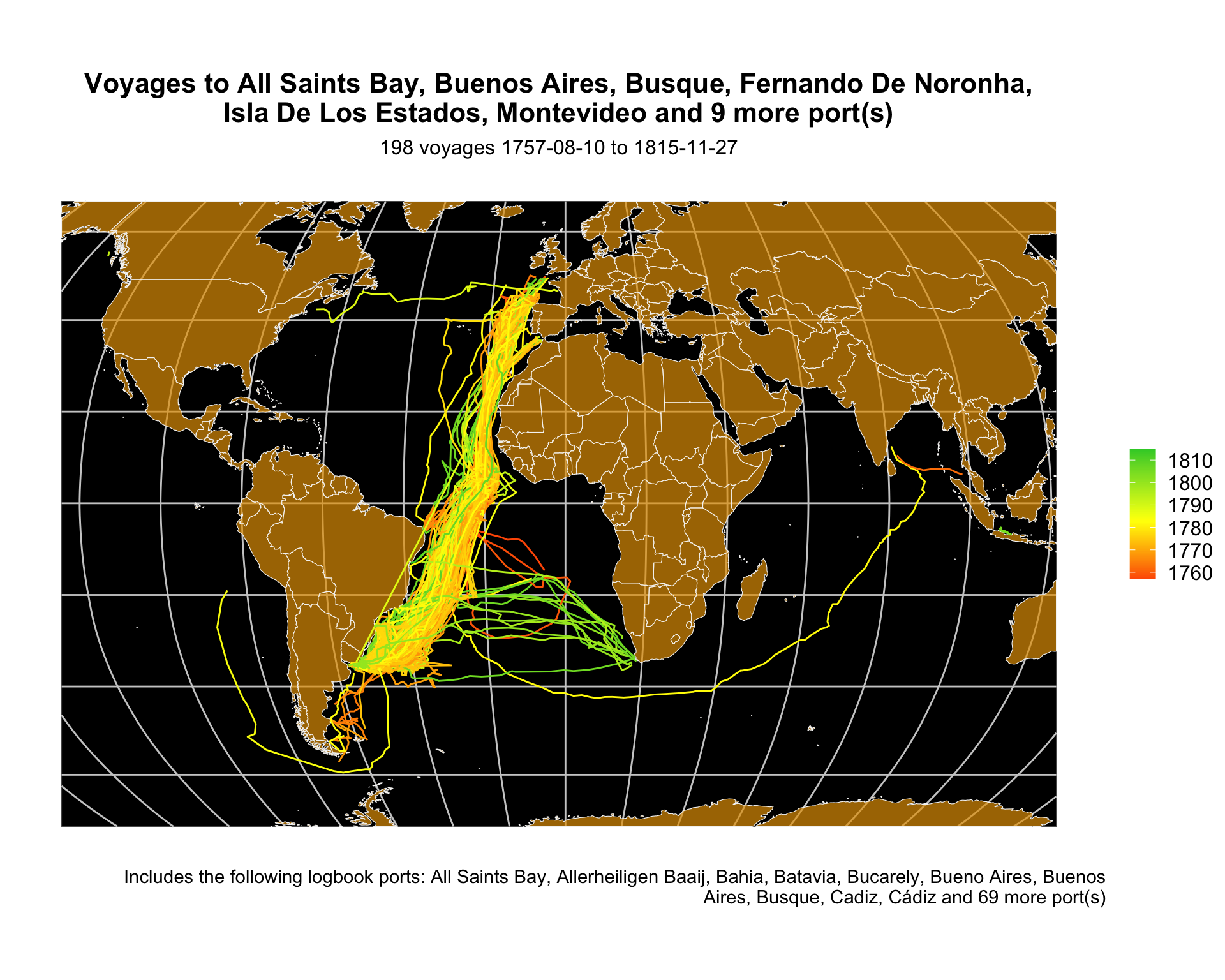
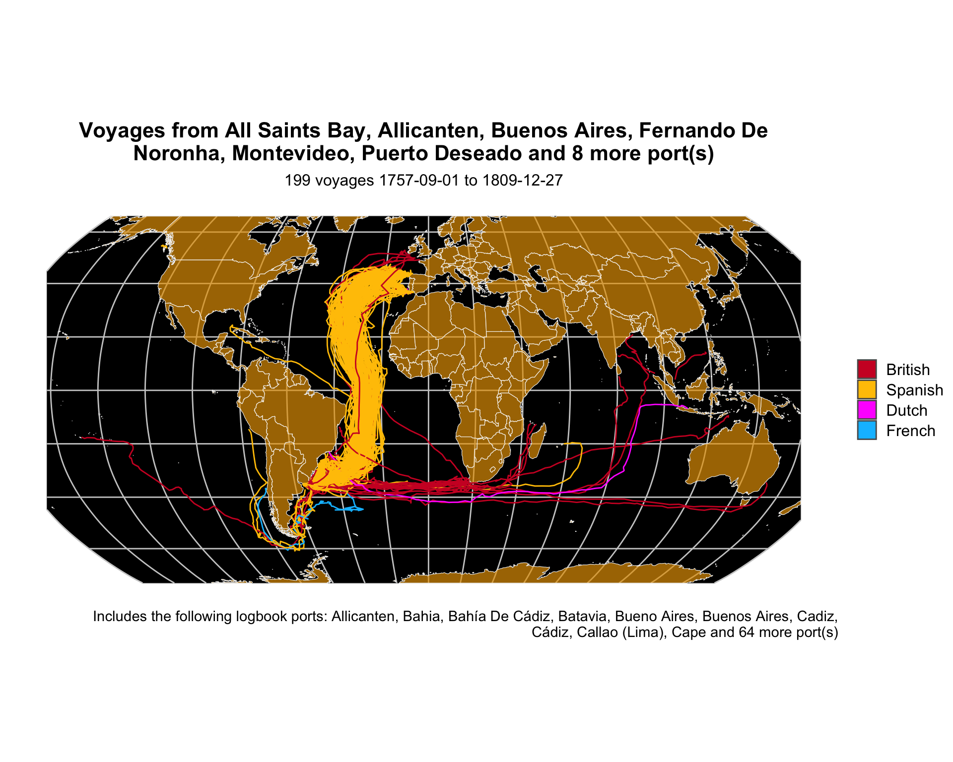
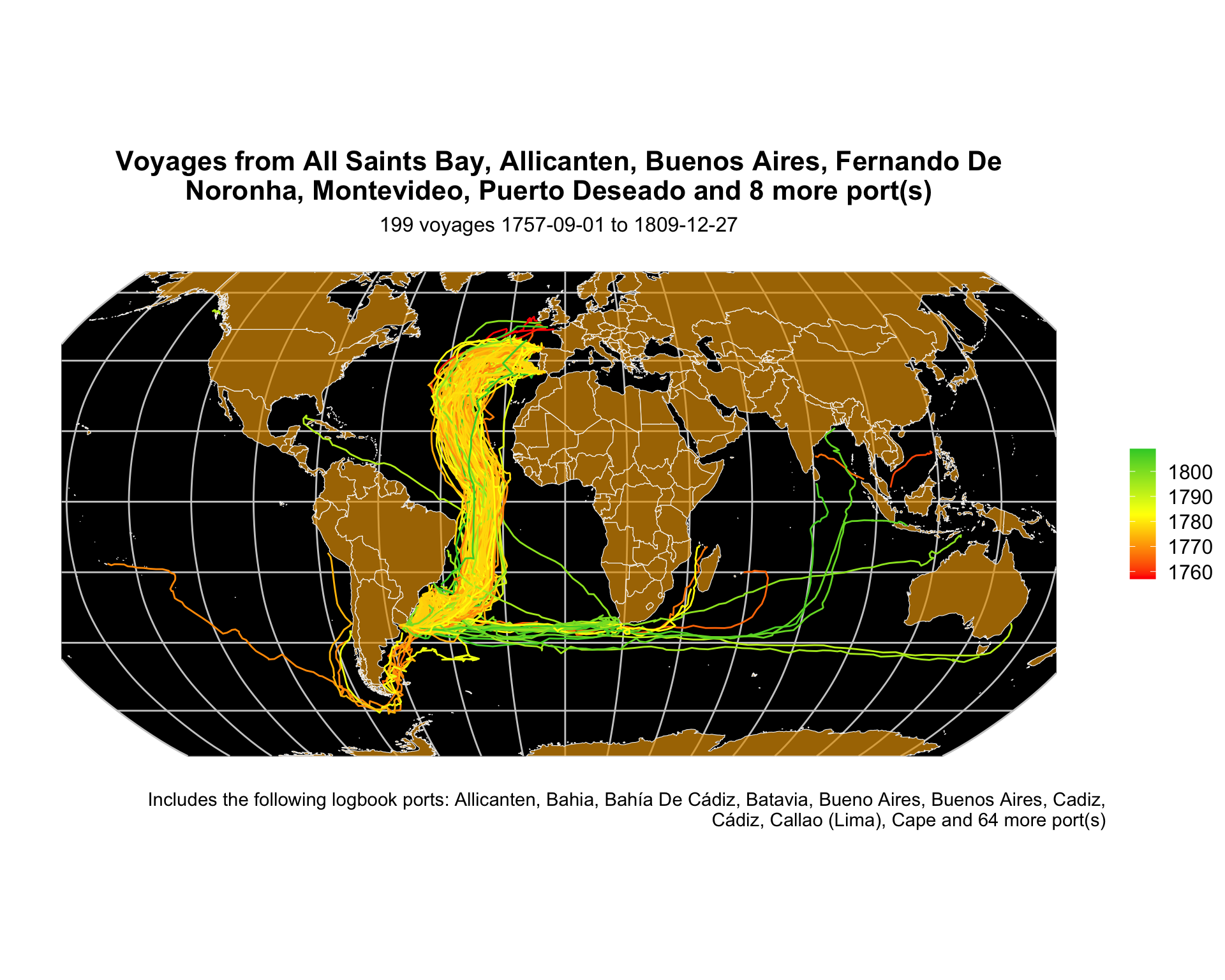
Most voyages in our data from or to South America we between to Montevideo and Spanish ports. Montevideo was Spain’ primary naval base in this period. The trade from the interior via the Río de la Plata (River Plate) passed through Montevideo or Buenos Aires, which sits on the opposite coast of the estuary.

At least some of the British voyages likely contributed to the Battle of Montevideo (1807) or its aftermath, when the British captured and held Montevideo for much of that year.

The voyages to or from Spain occurred before or during the 1780s–well before British blockades of Spanish ports 1797-1893 and 1803-1808.

Show the code
plot_voyages(to = df_voyages %>% 
      filter(country_to %in% c("brazil", "uruguay", "argentina" ))  %>%
      pull(port_to)
      )

plot_voyages(to = df_voyages %>% 
      filter(country_to %in% c("brazil", "uruguay", "argentina" ))  %>%
      pull(port_to),
      color_var = "year"
      )
Figure 2.18: All voyages to or from Spanish America
Figure 2.19: All voyages to or from Spanish America


Show the code
plot_voyages(from = df_voyages %>% 
      filter(country_from %in% c("brazil", "uruguay", "argentina" ))  %>%
      pull(port_from)
      )

plot_voyages(from = df_voyages %>% 
      filter(country_from %in% c("brazil", "uruguay", "argentina" ))  %>%
      pull(port_from),
      color_var = "year"
      )
Figure 2.20: All voyages from Spanish America
Figure 2.21: All voyages from Spanish America


2.3.2 The challenge of rounding the Horn traveling west

The track of the french ship La Boussole illustrates the difficulty square-rigged ships faced from storms and contrary winds.

Show the code
plot_voyages(from = df_voyages %>% 
      filter(country_from %in% c("brazil"),
             Nationality == "FRENCH")  %>%
      pull(port_from),
      ships = "LA BOUSSOLE"
      )
Figure 2.22: La Boussole’s track around the horn of South America
Show the code
plot_voyages(
      ships = "LA BOUSSOLE"
      )
Figure 2.23: La Boussole’s track around the horn of South America


2.4 Maps: African Guinea

2.4.1 Triangular trade

Show the code
guinea_coast <- c("senegal", "guinea-bissau", "guinea", "sierra leone", "liberia", "ivory coast", "ghana", "togo", "benin", "nigeria", "cameroon", "equatorial guinea", "gabon")

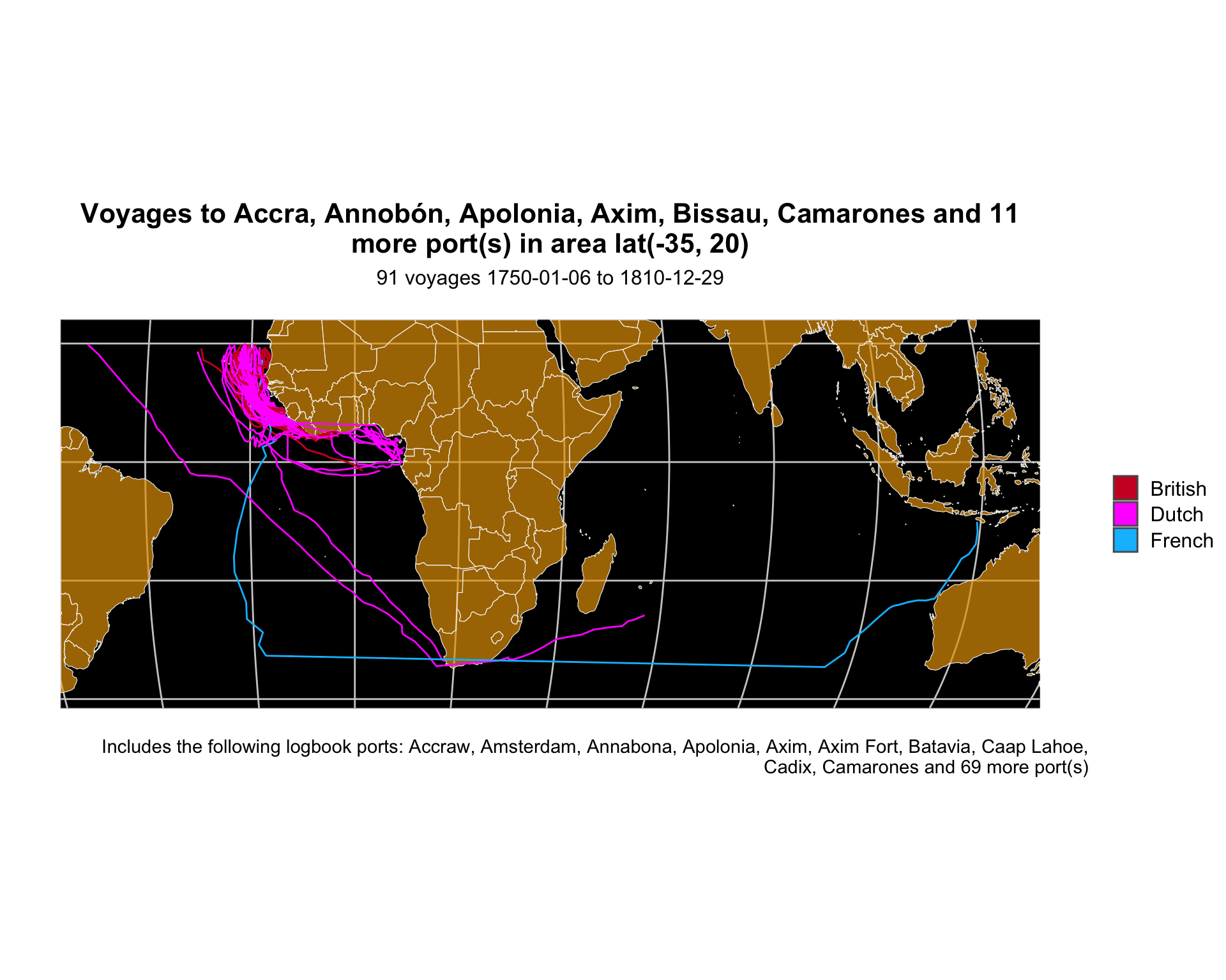
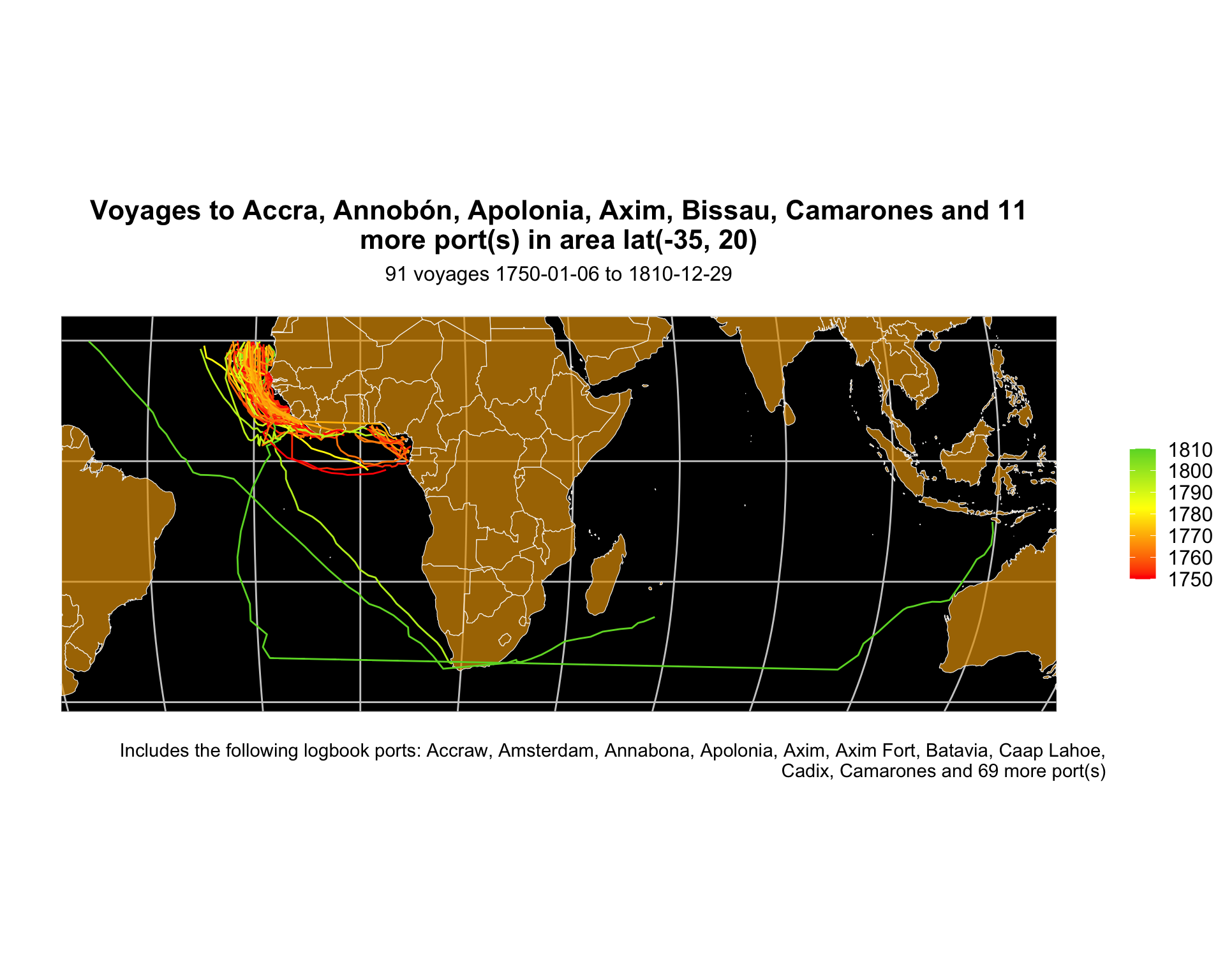
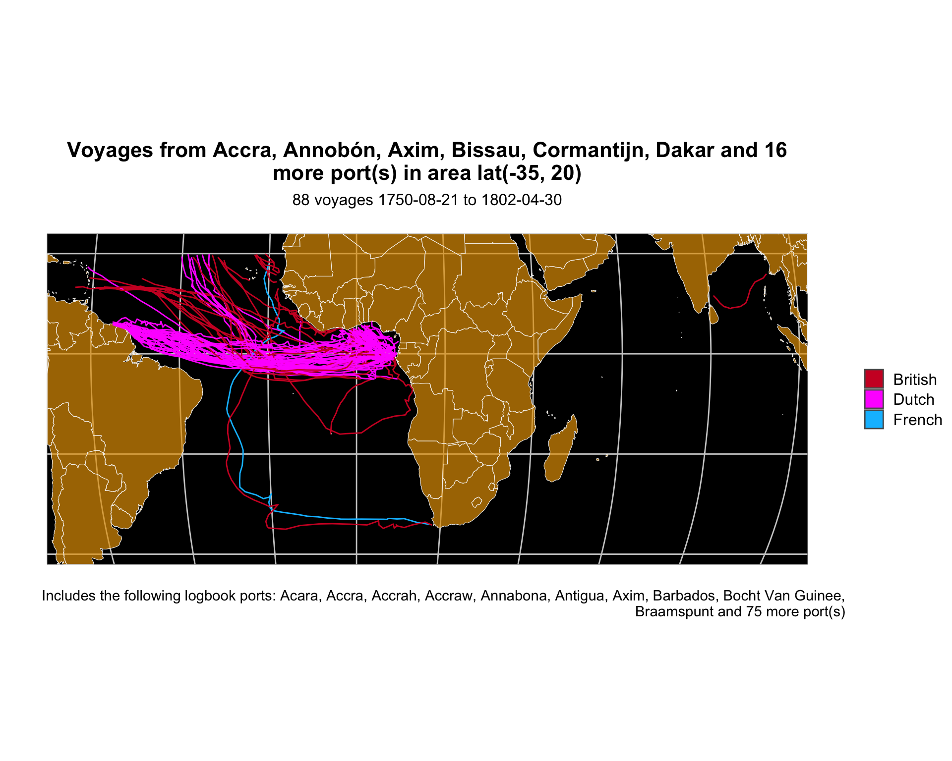
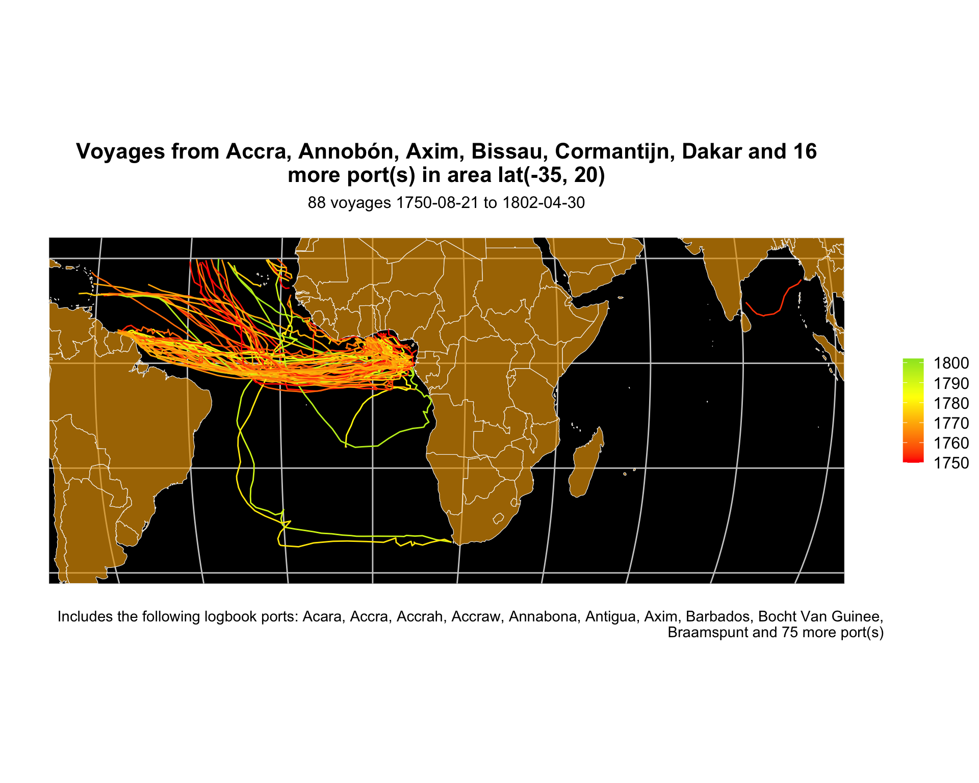
In our data set: Dutch and British voyages before 1780 to Guinea, modern day Senegal, Guinea-Bissau, Guinea, Sierra Leone, Liberia, Ivory Coast, Ghana, Togo, Benin, Nigeria, Cameroon, Equatorial Guinea and Gabon. Most voyages were to/from slave trading posts or colonial fortresses. We see two parts of the triangular trade route: from Europe to Guinea, then to the Americas.

Show the code
plot_voyages(to = df_voyages %>% 
      filter(country_to %in% guinea_coast)  %>%
      pull(port_to),
      range_lat = c(-35, 20)
      )

plot_voyages(to = df_voyages %>% 
      filter(country_to %in% guinea_coast)  %>%
      pull(port_to),
      range_lat = c(-35, 20),
      color_var = "year"
      )
Figure 2.24: Voyages to the Guinea coast
Figure 2.25: Voyages to the Guinea coast


Show the code
plot_voyages(from = df_voyages %>% 
      filter(country_from %in% guinea_coast)  %>%
      pull(port_from),
      range_lat = c(-35, 20)
      )

plot_voyages(from = df_voyages %>% 
      filter(country_from %in% guinea_coast)  %>%
      pull(port_from),
      range_lat = c(-35, 20),
      color_var = "year"
      )
Figure 2.26: Voyages from the Guinea coast
Figure 2.27: Voyages from the Guinea coast


2.5 Maps: India and Indonesia

2.5.1 To and from Penang, Malaysia

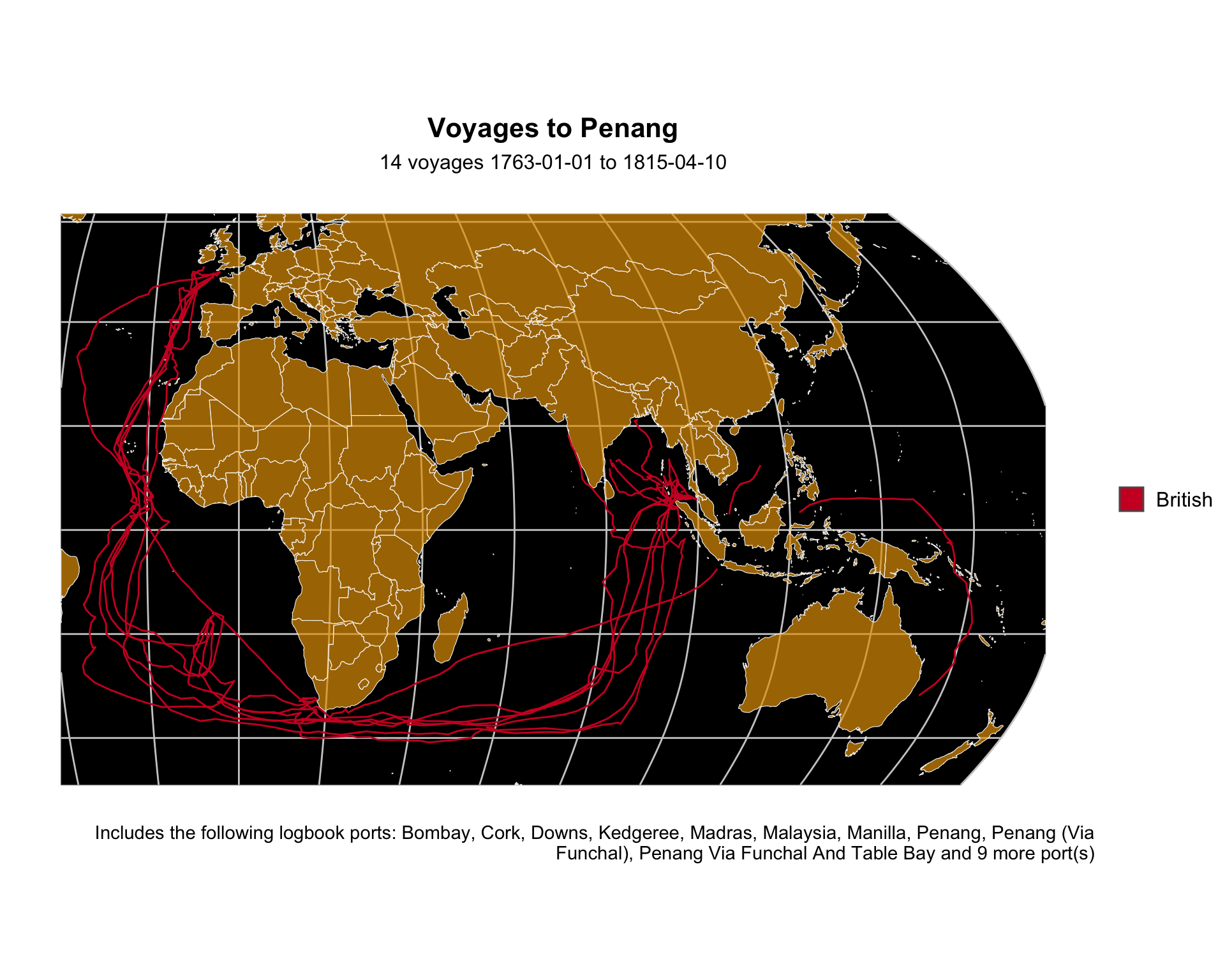
Our data set includes 28 voyages to or from Penang. There are just enough to see patterns in the routes: leaving the UK for Malaysia, ships stayed near Africa, veered toward Brazil, then picked up the prevailing westerlies beyond 35 degrees South, perhaps taking advantage of the Antarctic Circumpolar Current as well.

Show the code
plot_voyages(to = "penang")
Figure 2.28: Voyages to Penang, Malaya


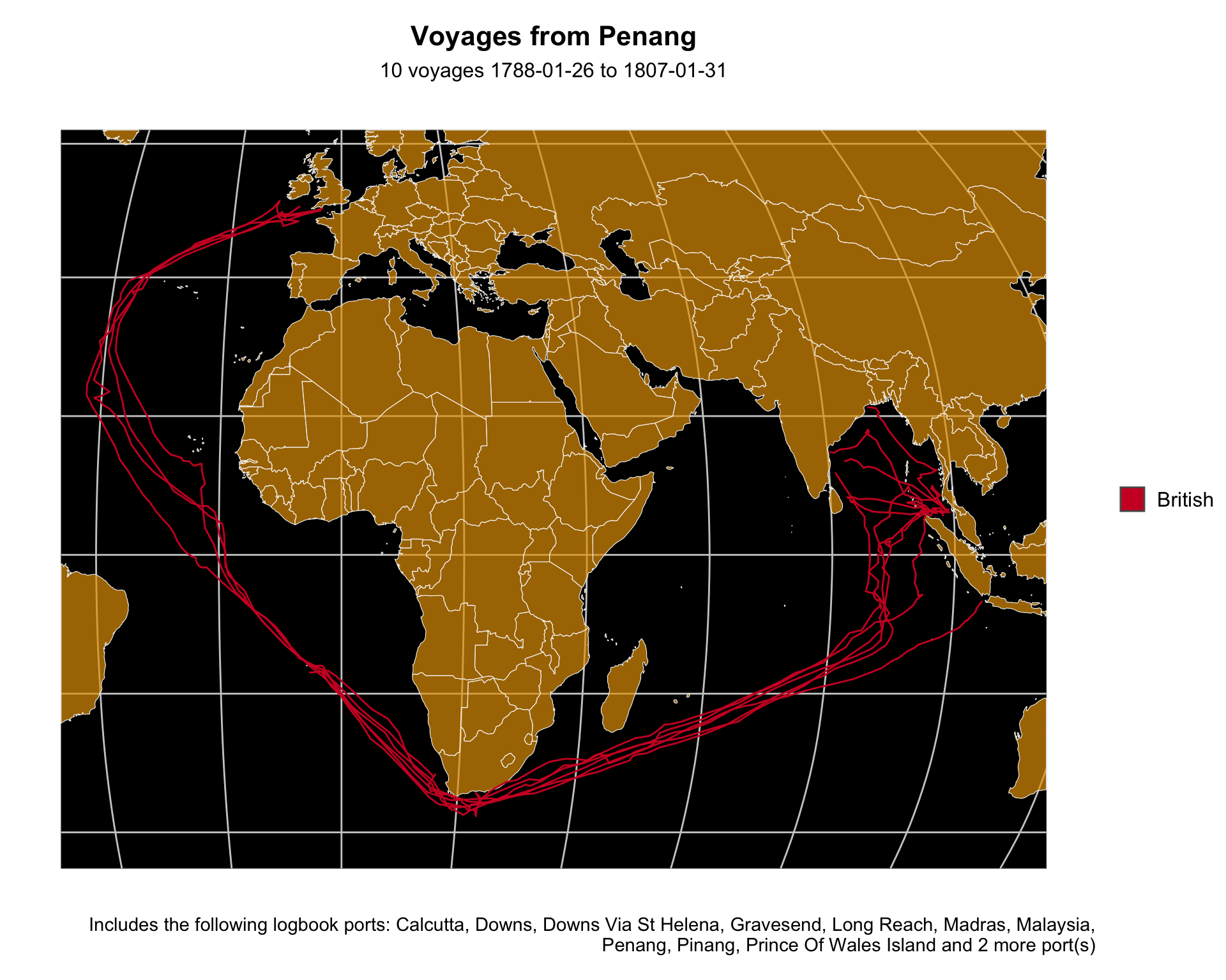
In contrast, when traveling the other direction, captains minimized the time they faced the prevailing westerlies, just barely rounding the Cape, then traveling much further into the north Atlantic before turning towards the UK.

Show the code
plot_voyages(from = "penang")
Figure 2.29: Voyages from Penang, Malaya


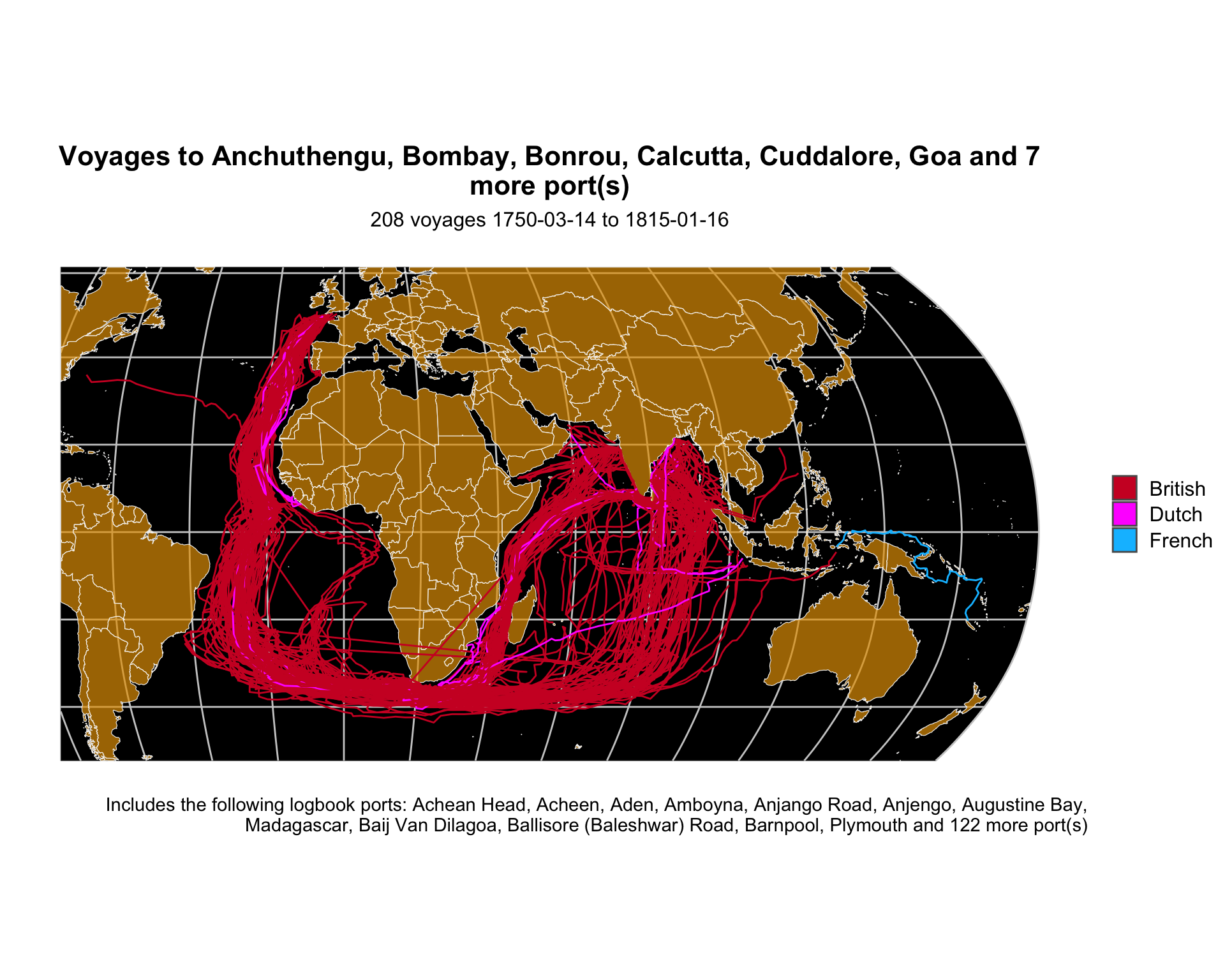
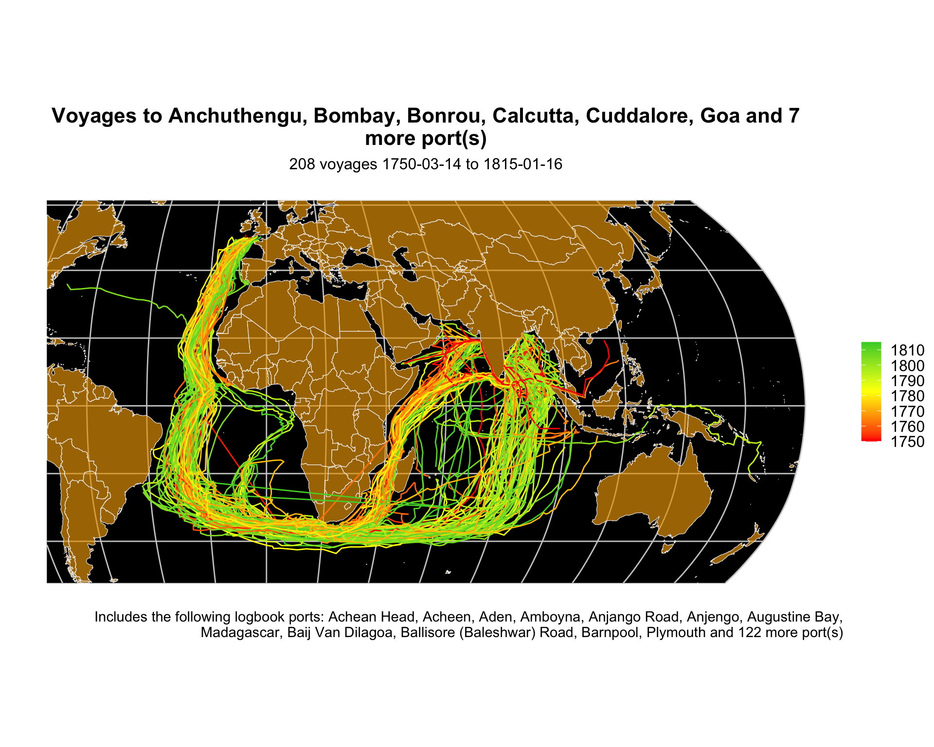
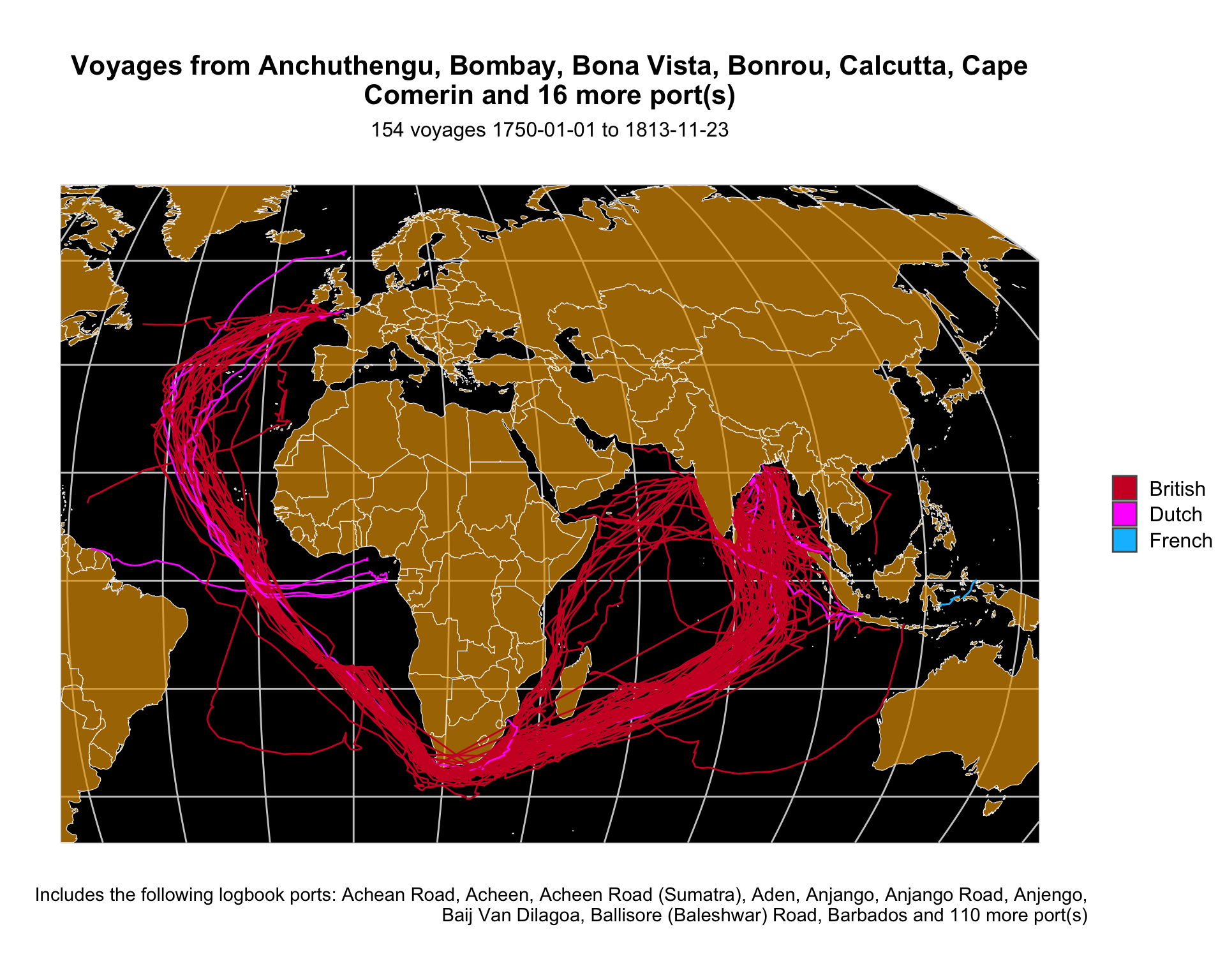
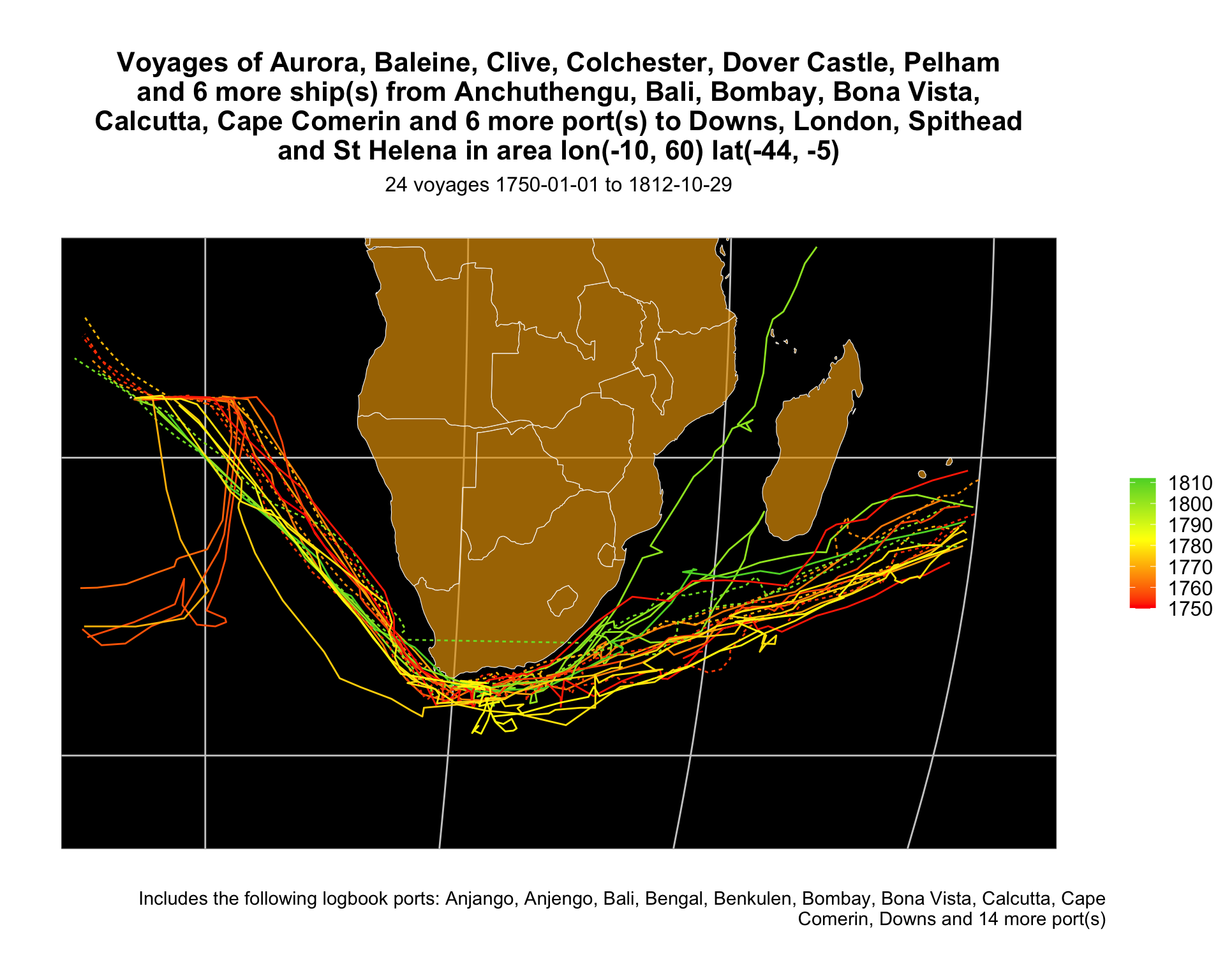
2.5.2 To and from India

This pattern is clearer still the tracks to and from India.

Show the code
plot_voyages(to = df_voyages %>%
               filter(country_to == "india") %>%
               pull(port_to)
)

plot_voyages(to = df_voyages %>%
               filter(country_to == "india") %>%
               pull(port_to),
             color_var = "year"
)
Figure 2.30: Voyages to India
Figure 2.31: Voyages to India


Show the code
plot_voyages(from = df_voyages %>%
               filter(country_from == "india") %>%
               pull(port_from)
)
Figure 2.32: Voyages from India


2.5.3 To and from Indonesia

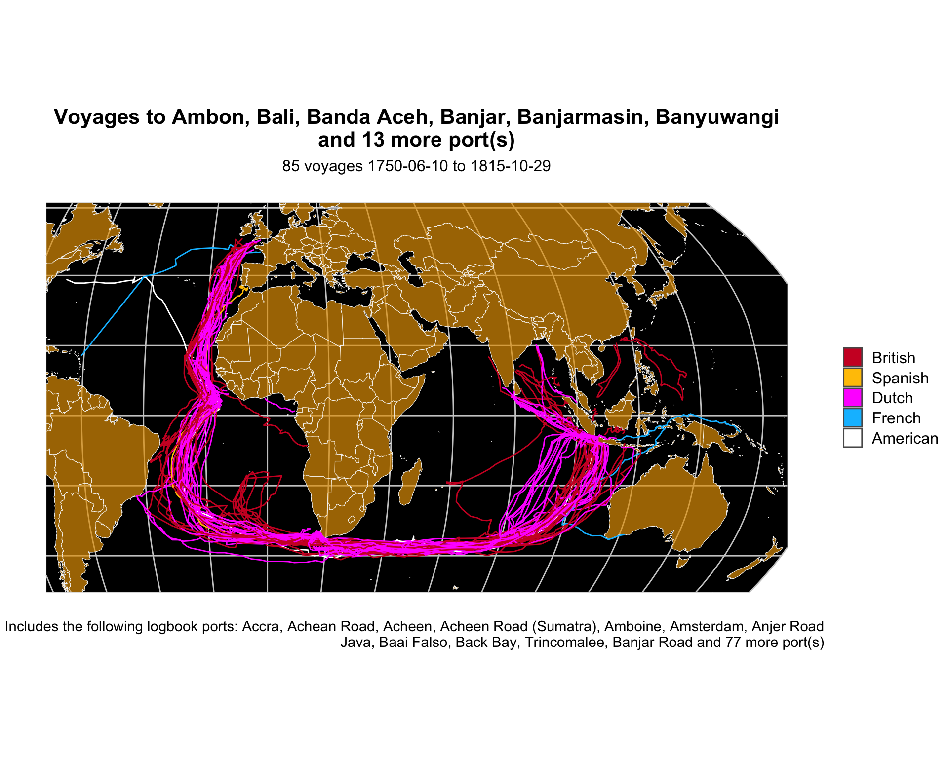
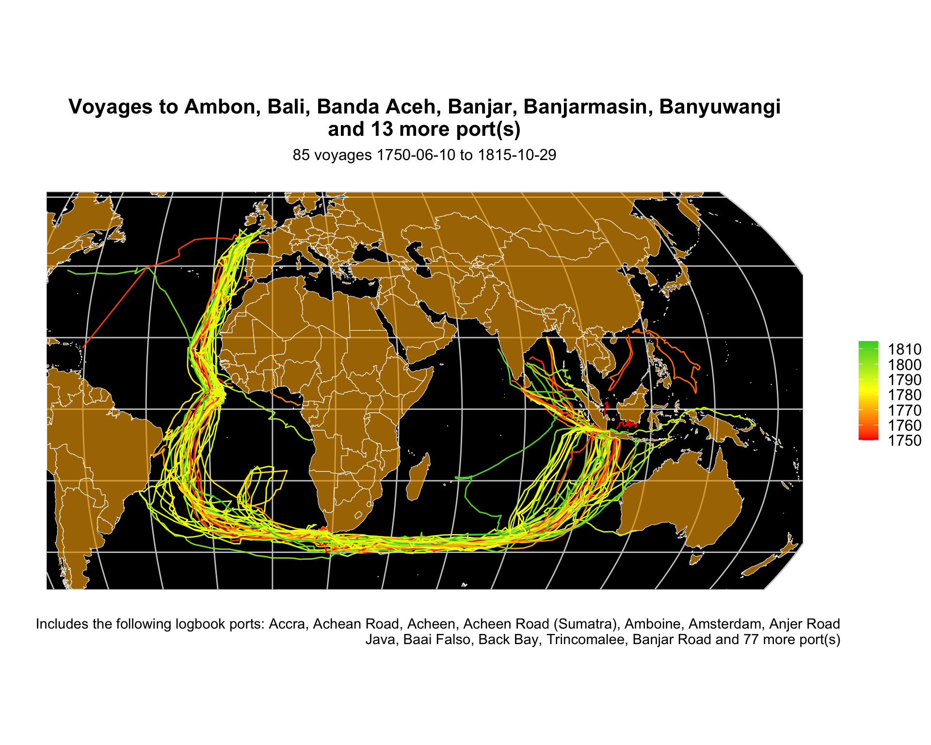
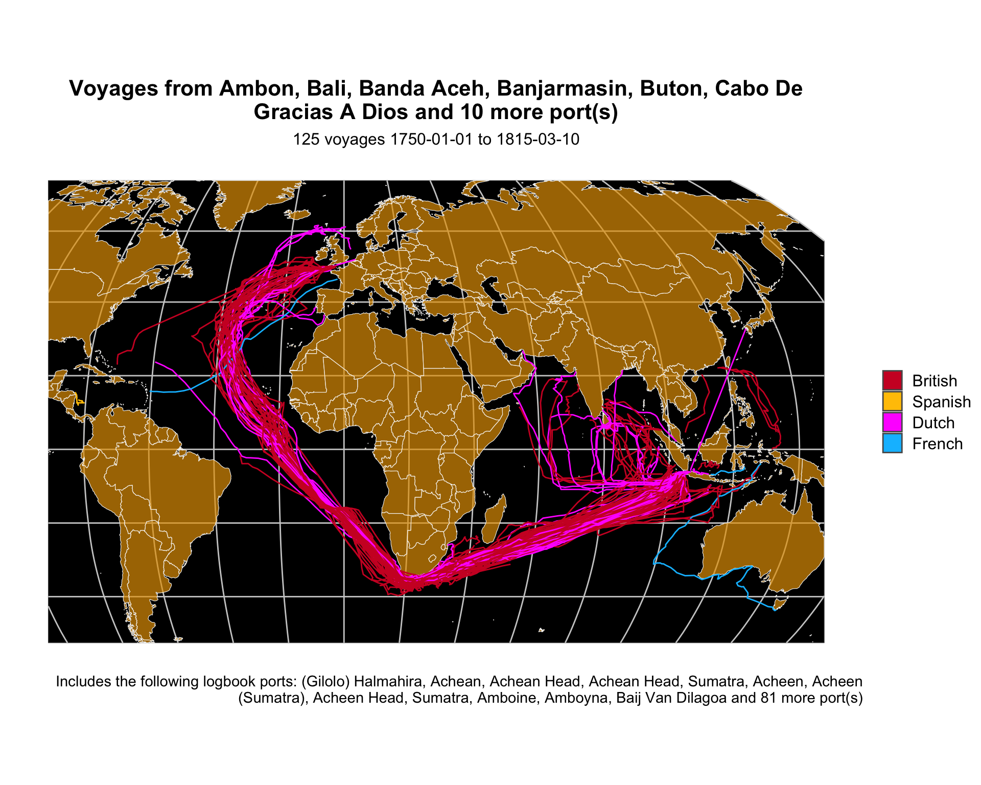
The same pattern is largely true for ships going to and from Indonesia. Most were Dutch; the main difference in their route was staying near 40 degrees South longer on the way to Indonesia.

Show the code
plot_voyages(to = df_voyages %>%
               filter(country_to == "indonesia") %>%
               pull(port_to)
)

plot_voyages(to = df_voyages %>%
               filter(country_to == "indonesia") %>%
               pull(port_to),
             color_var = "year"
)
Figure 2.33: Voyages to Indonesia
Figure 2.34: Voyages to Indonesia


Show the code
plot_voyages(from = df_voyages %>%
               filter(country_from == "indonesia") %>%
               pull(port_from)
)

plot_voyages(from = df_voyages %>%
               filter(country_from == "indonesia") %>%
               pull(port_from),
             color_var = "year"
)
Figure 2.35: Voyages from Indonesia
Figure 2.36: Voyages from Indonesia


2.5.4 To and from China

This data set includes only a small number voyages to or from Chinese ports.

Show the code
plot_voyages(to = df_voyages %>% filter(country_to == "china") %>% pull(port_to))
plot_voyages(to = df_voyages %>% filter(country_to == "china") %>% pull(port_to), color_var = "year")
Figure 2.37: Voyages to China
Figure 2.38: Voyages to China
Show the code
plot_voyages(from = df_voyages %>% filter(country_from == "china") %>% pull(port_from))
plot_voyages(from = df_voyages %>% filter(country_from == "china") %>% pull(port_from), color_var = "year")
Figure 2.39: Voyages from China
Figure 2.40: Voyages from China


2.6 The Importance of Chronometers

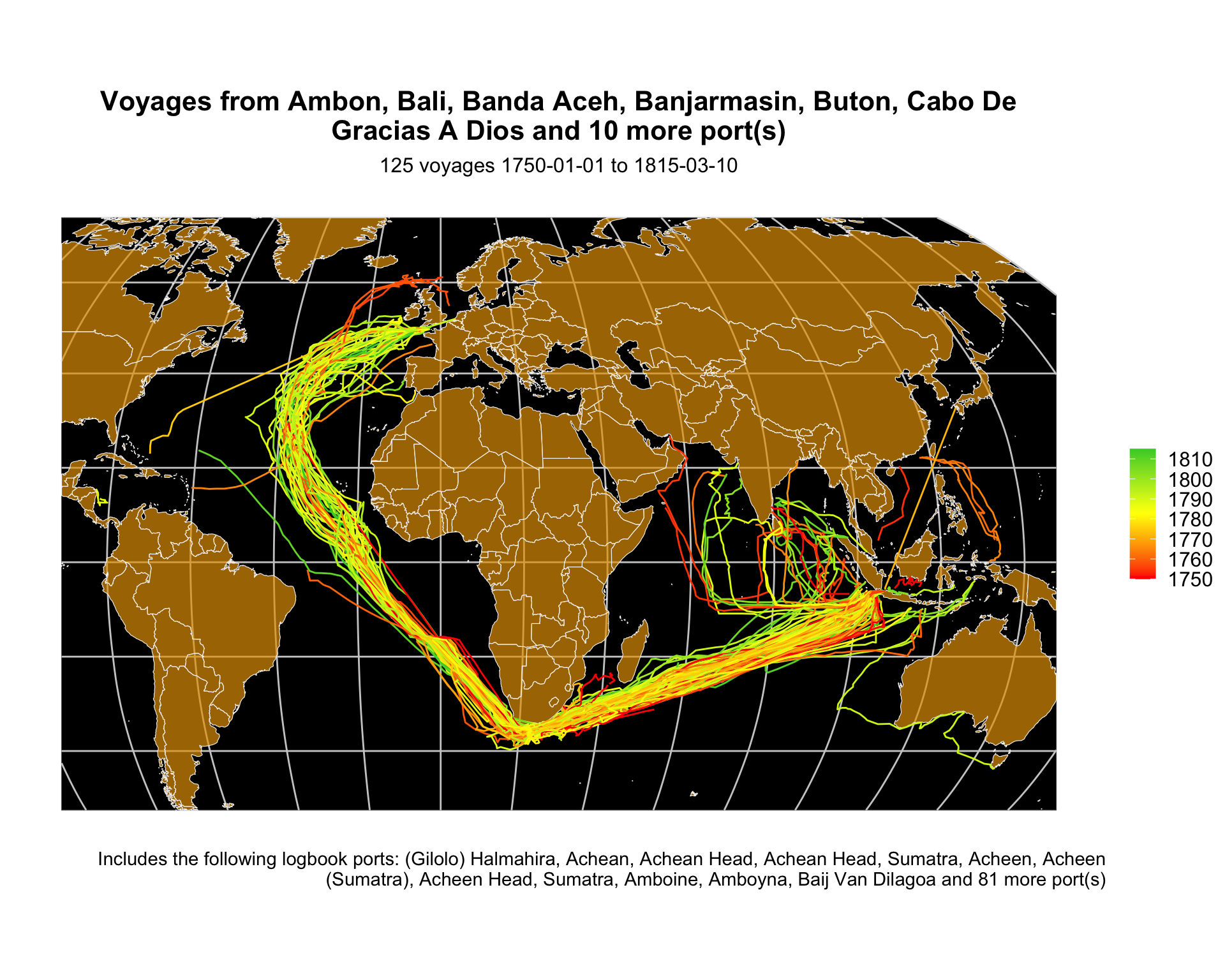
Perhaps you’ve noticed the unlikely number of horizontal tracks, for example, above when leaving Jakarta and traveling to western India or Yemen or ships approaching St Helena from the East. Ships would round the Cape and find the right latitude well to the east of St Helena. Then they could sail directly west to the island. Why? Because it’s hard to find a small island in a big ocean, and until there were sufficiently accurate chronometers, it was much easier to calculate an accurate latitude than longitude. In the period of this data set, chronometer technology improved a lot, and one can see in the trend towards lesser safety margin in later years.

Show the code
voyage_list <- df_voyages %>%
               filter(country_from == "india" & port_to == "st helena")

plot_voyages(ships = voyage_list$ShipName,
             from = voyage_list$port_from,
             to = "st helena", 
             range_lon = c(-10, 60),
             range_lat = c(-44, -5),
             color_var = "year"
)
Figure 2.41: As chronometers got better, captains could assume more accurate logitude calculations