2  FY3210 in context

FY3210 is one of over 2900 marks in these four counties.

2.1 Survey mark network

Show the code
ggplot() +
  geom_sf(data = nc_counties, color="black",
          fill = NA, size = 0.25) +
  geom_sf(data = nc_marks_counties |>
            filter(county %in% c("Orange", "Chatham", "Durham", "Wake")),
          #aes(color = ortho_ht), #* 3.28084 convert to ft
          size = 1, color = "white",
          show.legend = TRUE
          ) +
  geom_sf(data = nc_marks_counties |>
            filter(county %in% c("Orange", "Chatham", "Durham", "Wake")),
          aes(color = ortho_ht), #* 3.28084 convert to ft
          size = 0.5,
          show.legend = TRUE
          ) +
  geom_sf(data = nc_counties_border_union, color="black",
          fill = NA, size = 1) +
  scale_color_gradientn(colors = pal_dem_screen$hex,
                        # values = scales::rescale(pal_dem_screen$limit),
                        # limit = range(pal_dem_screen$limit),
                        # values = my_values,
                        limit = my_range,
                        na.value = "transparent",
  ) +
  theme(axis.text = element_blank(),
        axis.ticks = element_blank(),
        legend.position = c(0.9, 0.8)) +
  labs(
    title = "Survey mark 'network'",
    subtitle = glue("{comma(n_marks_counties)} marks in {n_counties} NC counties"),
    caption = my_caption
  )
Figure 2.1: Survey mark ‘network’


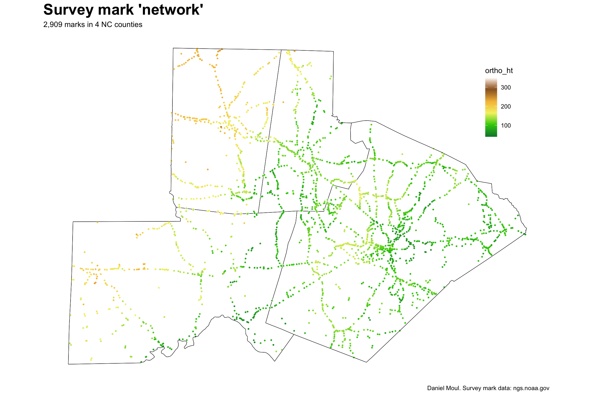
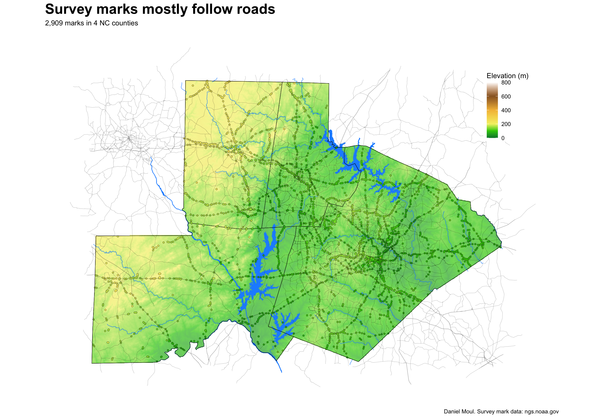
The geographical distribution of marks looks like a road network, because at least in these counties, survey marks are mostly located on or near roads.1

Show the code
ggplot() +
  geom_spatraster(data = elev_nc_counties,
                  alpha = 0.7) +
  geom_sf(data = nc_rivers, color = "dodgerblue", fill = "dodgerblue",
          linewidth = 0.25) +
  geom_sf(data = nc_waterbodies, color = "dodgerblue", fill = "dodgerblue",
          linewidth = 0.25) +
  geom_sf(data = nc_counties, color="black",
          fill = NA, size = 0.25) +
  geom_sf(data = nc_marks_counties,
          #aes(color = ortho_ht), #* 3.28084 convert to ft
          size = 0.75, color = "black", 
          # size = 1, color = "white",
          show.legend = TRUE
  ) +
  geom_sf(data = nc_marks_counties,
          aes(color = ortho_ht), #* 3.28084 convert to ft
          size = 0.5,
          show.legend = TRUE
          ) +
  geom_sf(data = nc_counties_border_union, color="black",
          fill = NA, size = 1) +
  geom_sf(data = streets$osm_lines,
          inherit.aes = FALSE,
          color = "black",
          #size = 0.05,
          linewidth = 0.075,
          alpha = 0.7) +
  scale_fill_gradientn(colors = pal_dem_screen$hex,
                       values = scales::rescale(pal_dem_screen$limit),
                       limit = range(pal_dem_screen$limit),
                       na.value = "transparent",
  ) +
  scale_color_gradientn(colors = pal_dem_screen$hex,
                        values = scales::rescale(pal_dem_screen$limit),
                        limit = range(pal_dem_screen$limit),
                        na.value = "transparent",
  ) +
  theme(axis.text = element_blank(),
        axis.ticks = element_blank(),
        legend.position = c(0.9, 0.8)
        ) +
  labs(
    title = "Survey marks mostly follow roads",
    subtitle = glue("{comma(n_marks_counties)} marks in {n_counties} NC counties"),
    caption = my_caption,
    color = "Elevation (m)",
    fill = "Elevation (m)"
  )
Figure 2.2: Survey marks mostly follow roads


2.2 Many kinds of marks

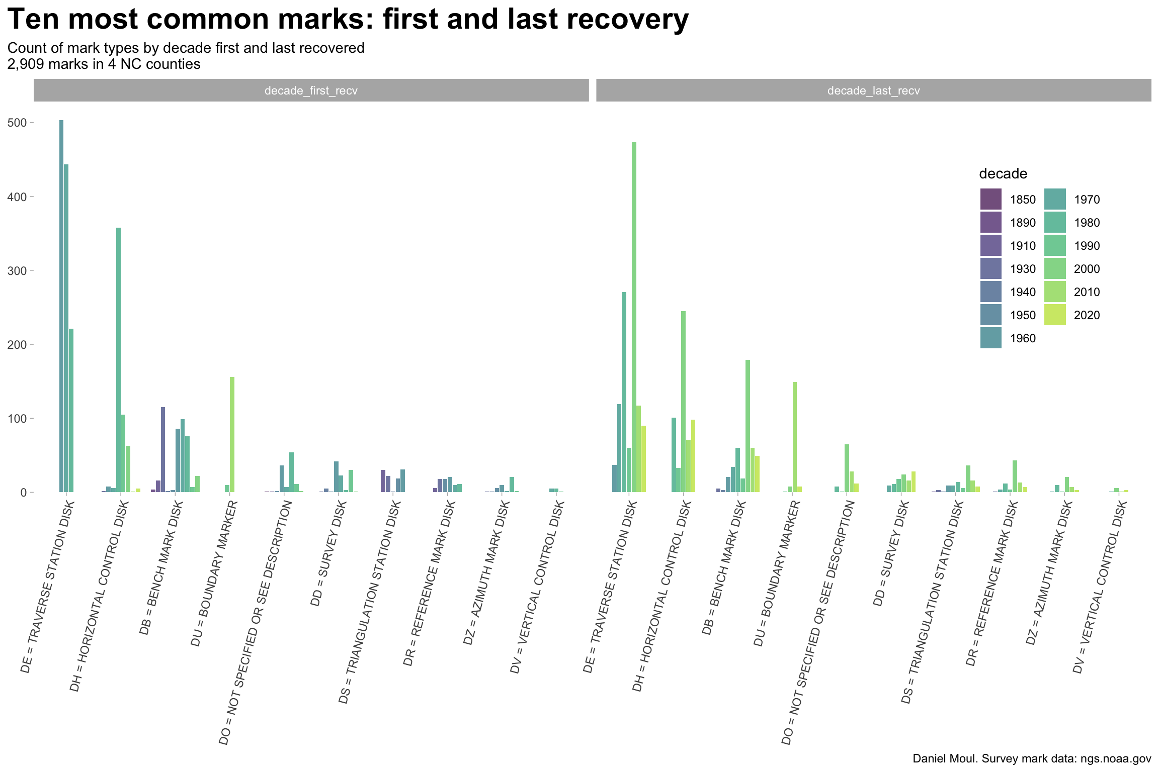
There are many kinds of marks (Section 6.4). The most common are marks determining horizontal location: Transverse Station marks and their predecessors Horizontal Control Disks, Reference Marks, and Boundary Marks. Vertical location marks include Bench Marks and Vertical Control Marks. There are many times more marks focused on horizontal location than elevation. Less common mark types are shown in Figure 6.1.

Show the code
data_for_plot <- nc_marks_counties |>
  st_drop_geometry() |>
  filter(!is.na(last_recv),
         !is.na(first_recv)) |>
  mutate(first_recv = as.numeric(str_extract(first_recv, "^[0-9]{4}")),
         last_recv = as.numeric(str_extract(last_recv, "^[0-9]{4}"))
         ) |>
  mutate(decade_first_recv = floor(first_recv / 10) * 10,
         decade_last_recv = floor(last_recv / 10) * 10) |>
  mutate(decade_last_recv = floor(last_recv / 10) * 10) |>
  replace_na(list(setting = "0 = UNSPECIFIED SETTING",
                  marker = "DO = NOT SPECIFIED OR SEE DESCRIPTION")) 

data_for_plot |>
  pivot_longer(cols = c(decade_first_recv, decade_last_recv),
               names_to = "first_or_last",
               values_to = "decade") |>
  count(first_or_last, decade, marker) |>
  arrange(decade) |>
  mutate(decade = as_factor(decade),
         marker = fct_reorder(marker, n, sum)
  ) |>
  mutate(marker = fct_lump_n(marker, w = n, n = 10)) |>
  filter(marker != "Other") |>
  mutate(marker = fct_rev(marker)) |>
  ggplot(aes(marker, n, fill = decade, group = first_or_last)) +
  geom_col(show.legend = TRUE,
           alpha = 0.7,
           position = position_dodge2(preserve = "single")) +
  scale_y_continuous(expand = expansion(mult = c(0, 0.05))) +
  scale_fill_viridis_d(end = 0.9) +
  guides(fill = guide_legend(ncol = 2)) +
  facet_wrap( ~first_or_last) +
  theme(legend.position = c(0.9, 0.6),
        axis.text.x = element_text(angle =75,
                                   hjust = 1)) +
  labs(
    title = "Ten most common marks: first and last recovery",
    subtitle = glue("Count of mark types by decade first and last recovered",
                    "\n{comma(n_marks_counties)} marks in {n_counties} NC counties"),
    x = NULL,
    y = NULL,
    caption = my_caption
  )
Figure 2.3: Survey and bench mark types: first and last recovery


2.3 Mark recovery activity

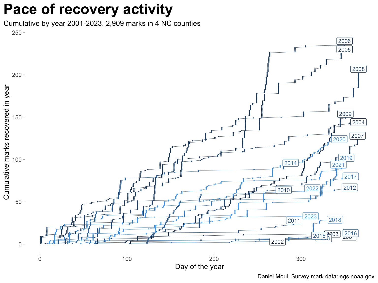
In recent years the last recovered date includes month and day, which reveals the varying amounts of activity in different years and the burstiness (near-vertical lines) in some years (Figure 2.4). Compare years of greatest activity with the densest sections of Figure 6.2 panel A.

Show the code
data_for_plot <- nc_marks_counties |>
  st_drop_geometry() |>
  mutate(last_rec_yday = yday(last_recv),
         year = year(last_recv),
         tmp = 1) |>
  filter(year > 2000) |>
  arrange(year, last_rec_yday) |>
    mutate(idx = row_number(),
           cum_mark = cumsum(tmp),
           .by = c(year))

data_for_plot_label <- data_for_plot |>
  filter(cum_mark == max(cum_mark),
         .by = year)

data_for_plot |>
  ggplot(aes(last_rec_yday, cum_mark, color = year, group = year)) +
  geom_line(linewidth = 0.15,
            show.legend = FALSE) + 
  geom_point(size = 0.2,
            show.legend = FALSE) +
  geom_label(data = data_for_plot_label,
            aes(label = year),
            size = 3,
            show.legend = FALSE) +
  labs(
    title = "Pace of recovery activity",
    subtitle = glue("Cumulative by year 2001-2023. {comma(n_marks_counties)} marks in {n_counties} NC counties"),
    x = "Day of the year",
    y = "Cumulative marks recovered in year",
    caption = my_caption
  )
Figure 2.4: Pace of recovery activity


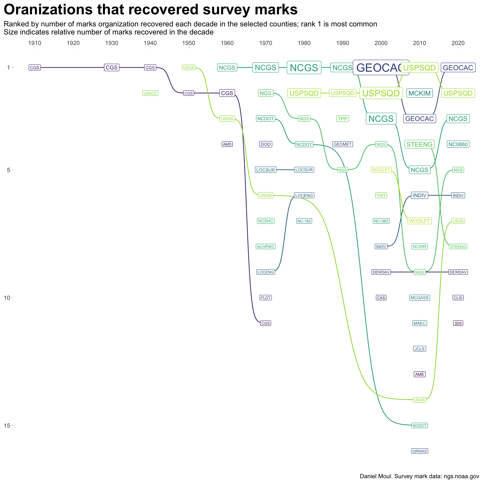
Marks have been recovered by public and private agencies, voluntary groups, and individuals. In each decade since 1980, in these in these four counties, voluntary groups (notably the U.S. Power Squadron) or other geocaching hobbyists have recovered the most marks, the second-most, or both (Figure 2.5).

Show the code
nc_marks_counties |>
  st_drop_geometry() |>
  filter(!is.na(last_recv),
         !is.na(last_recby),
         last_recby != "NONE") |>
  mutate(decade = floor(year(last_recv) / 10) * 10) |>
  count(decade, last_recby) |>
  group_by(decade) %>%
  mutate(decade_rank = nrow(cur_data()) - rank(n, ties.method = "first") + 1,
         last_recby_label = glue("{last_recby}: {n}")) |>
  ungroup() |>
  select(decade, last_recby, decade_rank, n, last_recby_label) |>
  ggplot(aes(decade, decade_rank, color = last_recby)) +
  geom_bump(show.legend = FALSE) +
  geom_point(show.legend = FALSE) +
  geom_label(aes(label = last_recby, size = n),
             show.legend = FALSE) +
  scale_x_continuous(position = "top",
                     breaks = 1910 + (0:11) * 10) +
  scale_size_continuous(range = c(2, 6)) +
  scale_y_reverse(breaks = c(1, 5, 10, 15, 20)) +
  scale_color_viridis_d(end = 0.9) +
  labs(
    title = "Oranizations that recovered survey marks",
    subtitle = glue("Ranked by number of marks organization recovered each decade in the selected counties; rank 1 is most common",
                    "\nSize indicates relative number of marks recovered in the decade"),
    x = NULL,
    y = NULL,
    caption = my_caption
  )
Figure 2.5: Oranizations ranked by number of recovered survey marks each decade


The U.S. Coast & Geodetic Survey (CGS) is now called the National Geodetic Survey (NGS).2 and is part of the National Ocean Service (still part of NOAA).

Table 2.1 includes the name associated with each abbreviation used in Figure 2.5 as well as total marks recovered in all decades.

Show the code
contrib |>
  select(last_recby_org, last_recby, n) |>
  arrange(last_recby_org) |>
  gt() |>
  tab_options(table.font.size = 10) |>
  tab_header(md(glue("**{n_org} organizations recovered survey marks**"))) |>
  tab_source_note(md("*Table: Daniel Moul; source: www.ngs.noaa.gov/cgi-bin/get_contrib2.prl retrieved 2024-02-03*"))
Table 2.1: Oranizations that recovered survey marks
35 organizations recovered survey marks
last_recby_org last_recby n
AERO-METRIC ENGINEERING INCORPORATED AME 2
CITY OF CHAPEL HILL NORTH CAROLINA NC0860 21
CITY OF DURHAM NORTH CAROLINA NC1360 1
CLARK LAND SURVEYING INCORPORATED CLSI 1
CONTINENTAL AERIAL SURVEY INCORPORATED CAS 1
DEWBERRY DAVIS DEWDAV 2
DIVERSIFIED DESIGN AND DRAFTING SERVICES INC 3DS 1
FLORIDA DEPARTMENT OF TRANSPORTATION FLDT 1
GEOCACHING GEOCAC 798
GEOMETRICS GPS INCORPORATED GEOMET 2
GRW AERIAL SURVEY GRWAS 1
INDIVIDUAL CONTRIBUTORS INDIV 23
JOHN CHANCE LAND SURVEYS INC JCLS 2
LOCAL ENGINEER (INDIVIDUAL OR FIRM) LOCENG 3
LOCAL SURVEYOR (INDIVIDUAL OR FIRM) LOCSUR 7
MA ENGINEERING CONSULTANTS, INCORPORATED MAEC 2
MCGILL AND ASSOCIATES MCGASS 2
MCKIM AND CREED MCKIM 83
NATIONAL GEODETIC SURVEY NGS 38
NORTH CAROLINA DEPARTMENT OF TRANSPORTATION NCDOT 12
NORTH CAROLINA GEODETIC SURVEY NCGS 1042
NORTH CAROLINA HIGHWAY AND PUBLIC WORKS COMM NCHPWC 1
NORTH CAROLINA STATE HIGHWAY COMMISSION NCSHC 2
NORTH CAROLINA WILDLIFE RESOURCES COMMISSION NCWR 3
STEWART ENGINEERING INC. STEENG 69
T P PARKER AND SON TPP 13
TAYLOR WISEMAN AND TAYLOR CONSULTING ENGINEERS TWT 2
US ARMY CORPS OF ENGINEERS USACE 1
US ARMY MAP SERVICE (NOW DMA) AMS 1
US COAST AND GEODETIC SURVEY (NOW NOS) CGS 68
US DEPARTMENT OF DEFENSE DOD 6
US GEOLOGICAL SURVEY USGS 12
US POWER SQUADRON USPSQD 672
WAKE COUNTY NORTH CAROLINA NC-183 1
WOOLPERT CONSULTANTS WOOLPT 13
Table: Daniel Moul; source: www.ngs.noaa.gov/cgi-bin/get_contrib2.prl retrieved 2024-02-03


TODO: add teaser for next chapter


  1. Figure 2.2 includes Open Street Map data for roads of type “motorway”, “trunk”, “primary”, “secondary”, “tertiary”, and “road”.https://wiki.openstreetmap.org/wiki/Key:highway ↩︎

  2. https://www.usgs.gov/faqs/how-can-i-find-survey-benchmark-and-triangulation-station-information ↩︎