1  Yearly output

There is great variation in the amount produced both over time and among the commodities. These dynamics are the focus of this chapter. Most mass units are metric tonnes (t). Gold and silver are measured in kg, and diamonds are measured in carets.


1.1 Contributions in 2021 to total amount extracted

Show the code
product_levels <- dta_yearly_long |>
  filter(year == 2021,
         !is.na(mass)) |>
  slice_max(order_by = mass, n = 1,
            by = product_mass) |>
  arrange(mass)

data_for_plot <- dta_yearly_long |>
  filter(year == 2021) |>
  select(year, mass, product_mass) |>
  inner_join(product_levels |> select(product_mass),
             by = "product_mass") |>
  mutate(product_mass = factor(product_mass, levels = product_levels$product_mass)) 

powers_of_ten <- round(log10(max(data_for_plot$mass) / min(data_for_plot$mass)))

In Figure 1.1 the range of output varies by 7 powers of 10: from 89 to 922,159,323.

Show the code
data_for_plot |>
  ggplot(aes(year, mass, label = product_mass, color = product_mass)) +
  geom_label_repel(na.rm = TRUE, show.legend = FALSE,
                   direction = "x", min.segment.length = 100000,
                   max.overlaps = 10, max.iter = 100000) +
  scale_x_continuous(breaks = c(1900, 1950, 2000)) +
  scale_y_log10(labels = label_number(scale_cut = cut_short_scale()),
  ) +
  labs(
    title = 'Australian mine output in 2021',
    x = NULL,
    y = "Amount (log10 scale)",
    caption = my_caption
  )

Figure 1.1: Amount extracted in 2021


1.2 Output per year by commodity

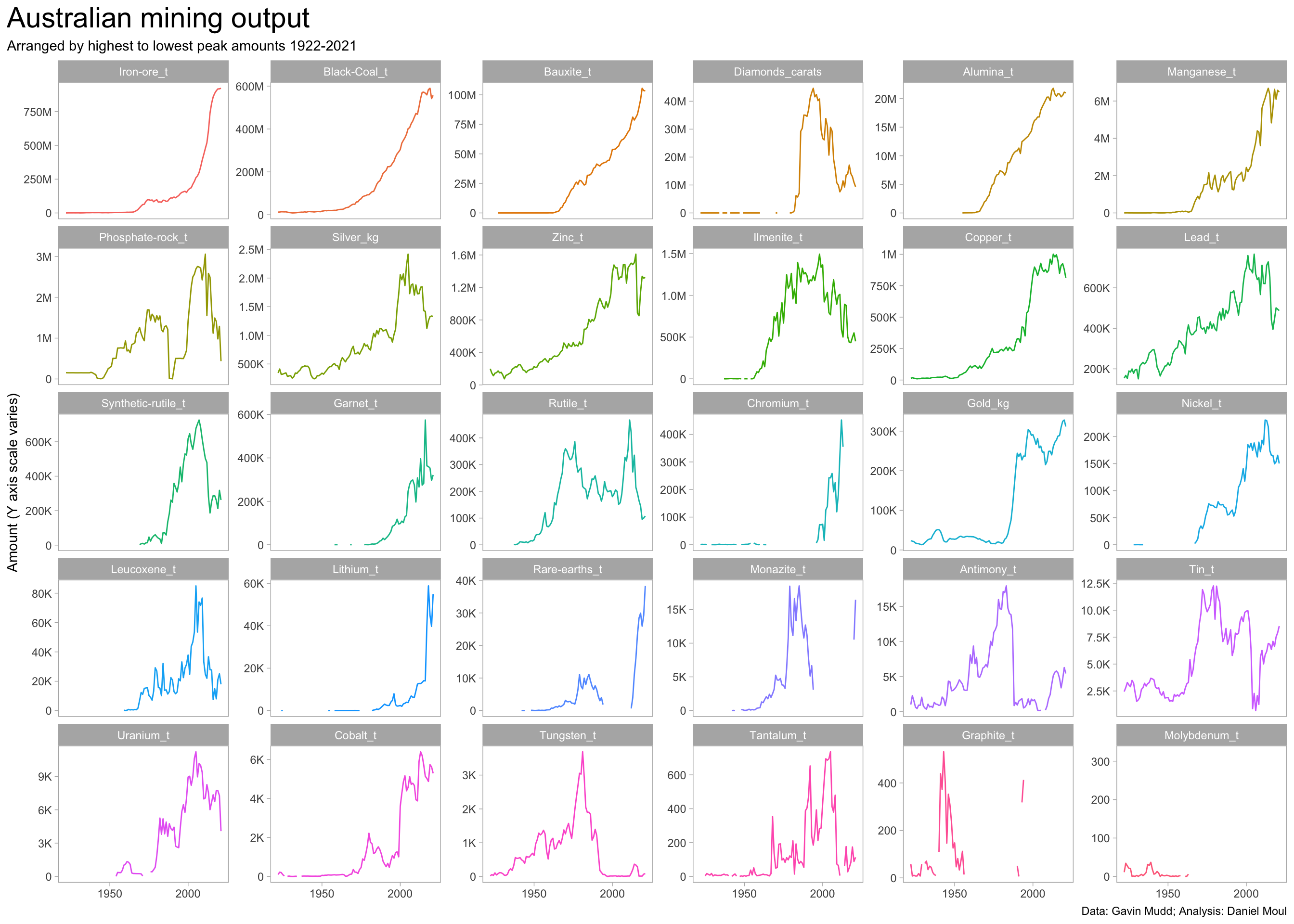
The output per year plots for each commodity is the sum of the output of all mines producing that commodity–which can vary significantly over short time periods. Mudd explains1:

The process of mining can be simplified to the following: mineral exploration finds a notable deposit of economic potential, approvals for mining are sought and obtained, the mine is built and begins operations, the deposit is eventually depleted or becomes uneconomic and the mine is closed and the site rehabilitated, and the cycle begins again …. Mining operations can be conducted through open pit or underground techniques, producing ‘ore’ which contains economic concentrations of the target metals or minerals as well as ‘waste rock’ with low to uneconomic concentrations of metals or minerals. The ore is processed to produce a saleable product such as a metal-rich concentrate (e.g., copper, nickel, lead, zinc or tin-rich concentrates), beneficiated mineral concentrate (e.g., saleable iron ore, beneficiated bauxite, washed coal) or metallic product (e.g., gold-silver doré bars, copper metal). After removal of the saleable product, the remaining minerals are called ‘tailings’ and are typically discharged to an engineered storage dam while waste rock is usually placed in large piles.

Show the code
product_levels <- dta_yearly_long |>
  filter(!is.na(mass)) |>
  slice_max(order_by = mass, n = 1,
            by = product_mass) |>
  arrange(desc(mass)) |>
  pull(product_mass)

dta_yearly_long |>
  mutate(product_mass = factor(product_mass, levels = product_levels)) |>
  ggplot(aes(year, mass, color = product_mass)) +
  geom_line(na.rm = TRUE, show.legend = FALSE) +
  scale_x_continuous(breaks = c(1900, 1950, 2000)) +
  scale_y_continuous(labels = label_number(scale_cut = cut_short_scale()),
  ) +
  facet_wrap(~ product_mass, scales = "free_y") +
  labs(
    title = glue("Australian mining output"),
    subtitle = glue("Arranged by highest to lowest peak amounts {year_first}-{year_last}"),
    x = NULL,
    y = "Amount (Y axis scale varies)",
    caption = my_caption
  )

Figure 1.2: Output over 100 years


1.3 Commodities at or near peak production levels

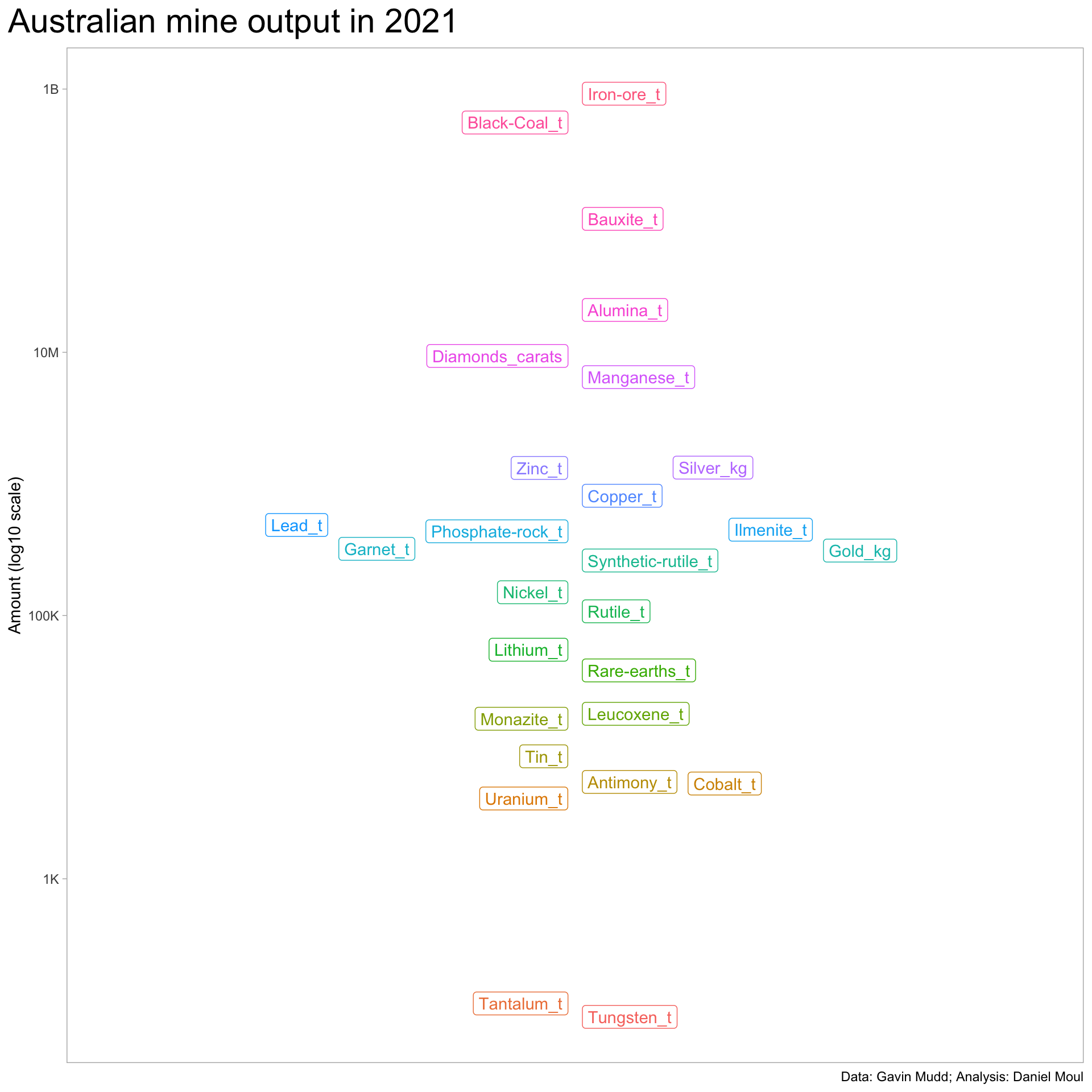
Production in 2021 was in the top 10% of historical peak production for the following commodities. Since the scale is so wide, I use a log scale on the Y axis.

Some observations:

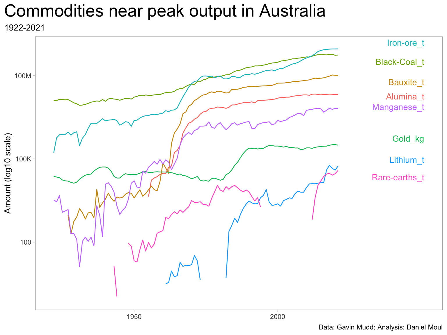
  • It’s distressing in these days of global warming that black coal production is near its peak. According to Geosciences Australia, a government agency, Japan is the the destination of more Australian coal then any other country, followed by China (assuming post-COVID-19 industrial activity returns to trend), then India, South Korea, and Taiwan. See Figure 92.
  • The main use of Bauxite and Alumina is in aluminium smelting. Another name for alumina is aluminium oxide (\(Al_2O_3\)) and Aluminium(III) oxide3. In North American English aluminium is aluminum.
  • Given the insatiable demand for batteries and magnets for electric vehicles and other electronic applications, it’s not surprising that mining of lithium and rare earth elements has increased dramatically over the last 30-40 years.
Show the code
peak_products <- dta_yearly_long |>
  filter(year == max(year, na.rm = TRUE) & mass >= mass_max * peak_production_cutoff) 

data_for_plot <- dta_yearly_long |>
  inner_join(peak_products %>% select(product_mass),
             by = "product_mass")

labels_for_plot <- data_for_plot |>
  filter(!is.na(mass)) |>
  mutate(final_year = max(year),
         .by = product_mass) |>
  filter(year == max(year),
         .by = product_mass)
  
data_for_plot |>
  ggplot(aes(year, mass, color = product_mass, group = product_mass)) +
  geom_line(na.rm = TRUE, show.legend = FALSE) +
  geom_text_repel(data = labels_for_plot,
                  aes(max(year) + 30, mass, label = product_mass),
                  hjust = 1, vjust = 0.5, show.legend = FALSE, 
                  direction = "y", force = 0.4) +
  scale_x_continuous(breaks = c(1850, 1900, 1950, 2000)) +
  scale_y_log10(labels = label_number(scale_cut = cut_short_scale()),
                limits = c(1, NA)) +
  labs(
    title = glue("Commodities near peak output in Australia"),
    subtitle = glue("{year_first}-{year_last}"),
    x = NULL,
    y = "Amount (log10 scale)",
    caption = my_caption
  )

Figure 1.3: Products at or near peak production: yearly Australian mining output


1.4 Table

Show the code
dta_yearly_long |>
  filter(year == 2021) |> 
  select(product_name, units_mass, mass, mass_max, mass_pct_of_max) |>
  arrange(desc(mass), desc(mass_max)) |>
  mutate(cum_pct = cumsum(mass / sum(mass, na.rm = TRUE)),
         rowid = row_number()) |>
  gt() |>
  tab_header(md("**Australian mining output 2021**")) |>
  fmt_number(columns = c(mass, mass_max),
             decimals = 0,
             suffixing = TRUE) |>
  fmt_percent(columns = mass_pct_of_max,
             decimals = 0) |>
  fmt_percent(columns = cum_pct,
             decimals = 2) |>
  sub_missing() |>
  tab_source_note(md("*Data: Gavin Mudd. Analysis: Daniel Moul*"))
Table 1.1: Australian mining output 2021
Australian mining output 2021
product_name units_mass mass mass_max mass_pct_of_max cum_pct rowid
Iron-ore t 922M 922M 100% 56.74% 1
Black-Coal t 557M 590M 94% 91.00% 2
Bauxite t 103M 106M 98% 97.36% 3
Alumina t 21M 22M 96% 98.65% 4
Diamonds carats 9M 45M 21% 99.22% 5
Manganese t 6M 7M 97% 99.62% 6
Silver kg 1M 2M 55% 99.70% 7
Zinc t 1M 2M 82% 99.79% 8
Copper t 813K 1M 81% 99.84% 9
Lead t 488K 766K 64% 99.87% 10
Ilmenite t 449K 1M 30% 99.89% 11
Phosphate-rock t 436K 3M 14% 99.92% 12
Garnet t 321K 575K 56% 99.94% 13
Gold kg 312K 328K 95% 99.96% 14
Synthetic-rutile t 262K 726K 36% 99.97% 15
Nickel t 150K 231K 65% 99.98% 16
Rutile t 108K 467K 23% 99.99% 17
Lithium t 55K 59K 94% 99.99% 18
Rare-earths t 38K 38K 100% 100.00% 19
Leucoxene t 18K 85K 21% 100.00% 20
Monazite t 16K 18K 89% 100.00% 21
Tin t 9K 12K 70% 100.00% 22
Antimony t 5K 18K 30% 100.00% 23
Cobalt t 5K 6K 83% 100.00% 24
Uranium t 4K 11K 36% 100.00% 25
Tantalum t 113 736 15% 100.00% 26
Tungsten t 89 4K 2% 100.00% 27
Chromium t 452K 28
Graphite t 531 29
Molybdenum t 324 30
Data: Gavin Mudd. Analysis: Daniel Moul


  1. https://www.nature.com/articles/s41597-023-02275-z ↩︎

  2. https://www.ga.gov.au/digital-publication/aecr2022/coal ↩︎

  3. https://www.britannica.com/science/alumina ↩︎