There is great variation in the value of the commodities produced over the years and among the minerals/metals. These dynamics are the focus of this chapter.
Value is \(price \times quantity\) .
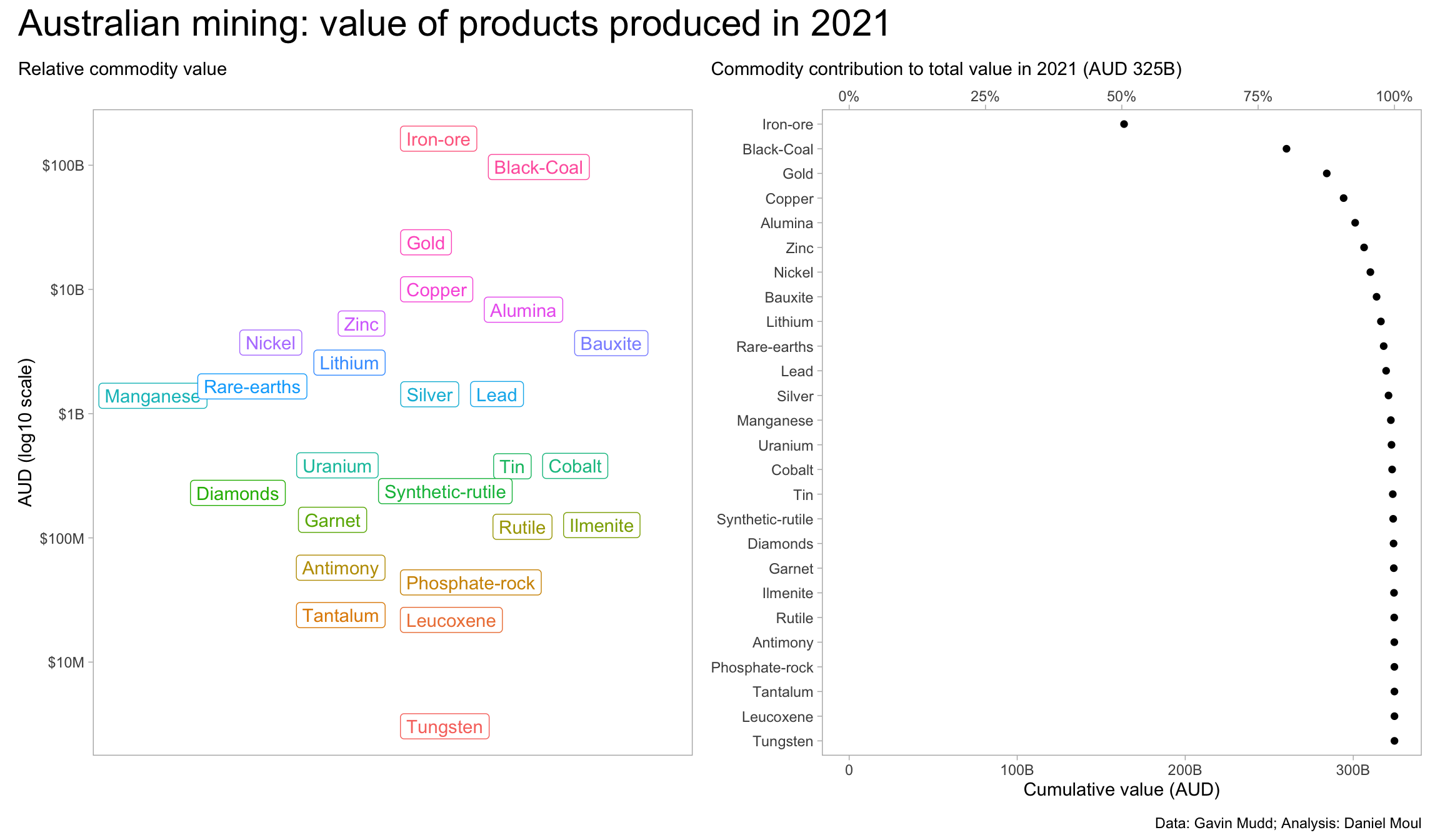
Contributions in 2021 to total value
Using log scale since the range is very wide.
Show the code
<- dta_yearly_long |> filter (year == 2021 ,! is.na (value_2021)) |> slice_max (order_by = value_2021, n = 1 ,by = product_name) |> arrange (value_2021)<- dta_yearly_long |> filter (year == 2021 ) |> inner_join (product_levels |> select (product_name),by = "product_name" ) |> mutate (product_name = factor (product_name, levels = product_levels$ product_name)) |> ggplot (aes (year, value_2021, label = product_name, color = product_name)) + geom_label_repel (na.rm = TRUE , show.legend = FALSE ,direction = "x" , min.segment.length = 100 ) + scale_x_continuous (breaks = c (1900 , 1950 , 2000 )) + scale_y_log10 (labels = label_number (scale_cut = cut_short_scale (),prefix = "$" ),+ labs (subtitle = glue ("Relative commodity value" ),x = NULL ,y = "AUD (log10 scale)" <- dta_yearly_long |> filter (year == 2021 ) |> inner_join (product_levels |> select (product_name),by = "product_name" ) |> arrange (desc (value_2021)) |> mutate (product_name = factor (product_name, levels = product_levels$ product_name),cum_value = cumsum (value_2021))= max (data_for_plot$ cum_value)<- data_for_plot |> ggplot (aes (cum_value, product_name)) + #geom_path(aes(group = cum_value), alpha = 0.4, color = carolina_blue) + geom_point () + scale_x_continuous (labels = label_number (scale_cut = cut_short_scale ()),sec.axis = sec_axis (~ . / max_cum_value,labels = label_percent (accuracy = 1 ))) + expand_limits (x = 0 ) + labs (subtitle = glue ("Commodity contribution to total value in 2021 (AUD {round(max_cum_value / 1e9, digits = 0)}B)" ),x = "Cumulative value (AUD)" ,y = NULL + p2 + plot_annotation (title = 'Australian mining: value of products produced in 2021' ,caption = my_caption
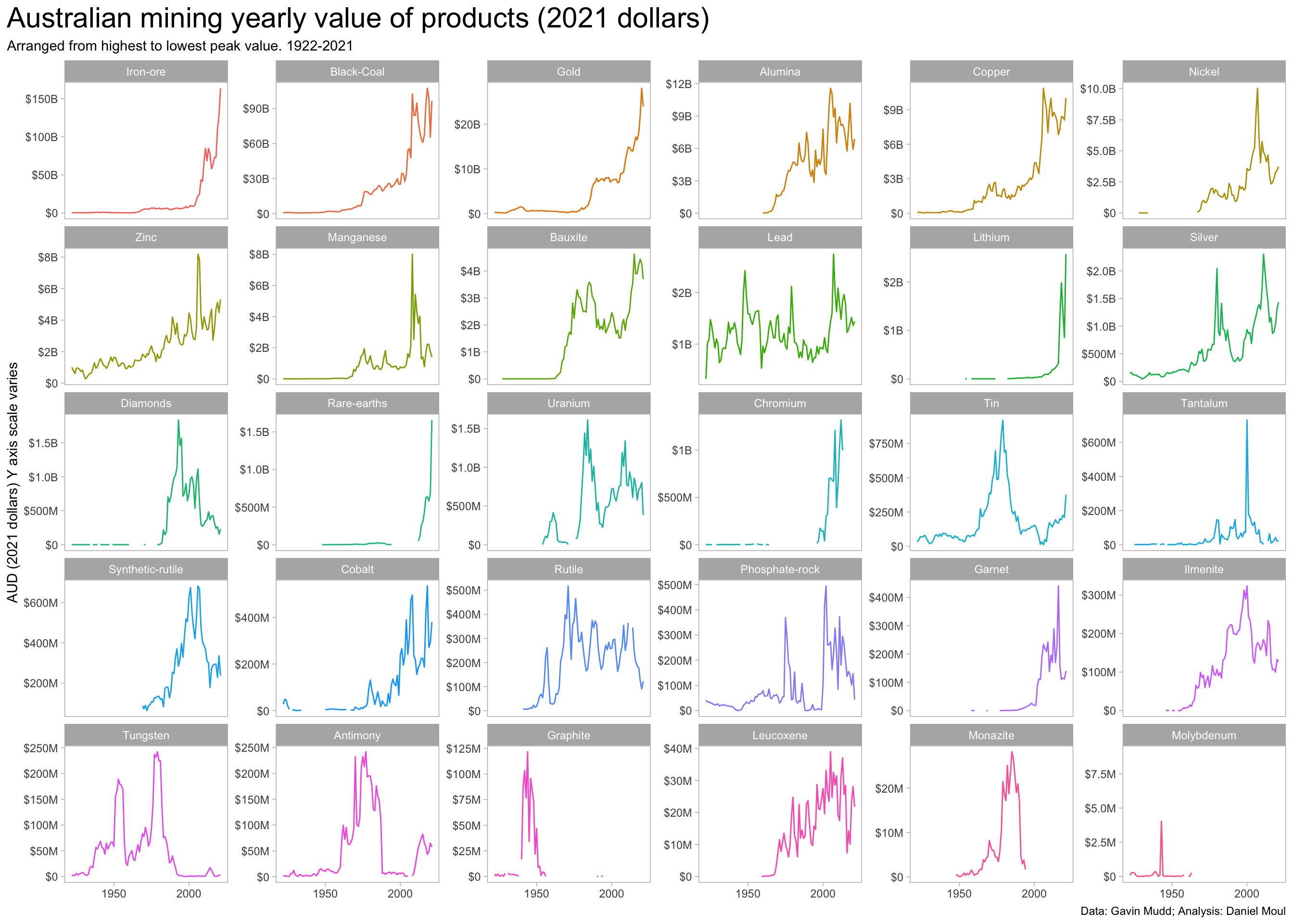
Yearly value by commodity
Show the code
<- dta_yearly_long |> filter (! is.na (value_2021)) |> slice_max (order_by = value_2021, n = 1 ,by = product_name) |> arrange (desc (value_2021)) |> pull (product_name)|> mutate (product_name = factor (product_name, levels = product_levels)) |> ggplot (aes (year, value_2021, color = product_name)) + geom_line (na.rm = TRUE , show.legend = FALSE ) + scale_x_continuous (breaks = c (1900 , 1950 , 2000 )) + scale_y_continuous (labels = label_number (scale_cut = cut_short_scale (),prefix = "$" ),+ facet_wrap (~ product_name, scales = "free_y" ) + labs (title = glue ("Australian mining yearly value of products (2021 dollars)" ),subtitle = glue ("Arranged from highest to lowest peak value. {year_first}-{year_last}" ),x = NULL ,y = "AUD (2021 dollars) Y axis scale varies" ,caption = my_caption
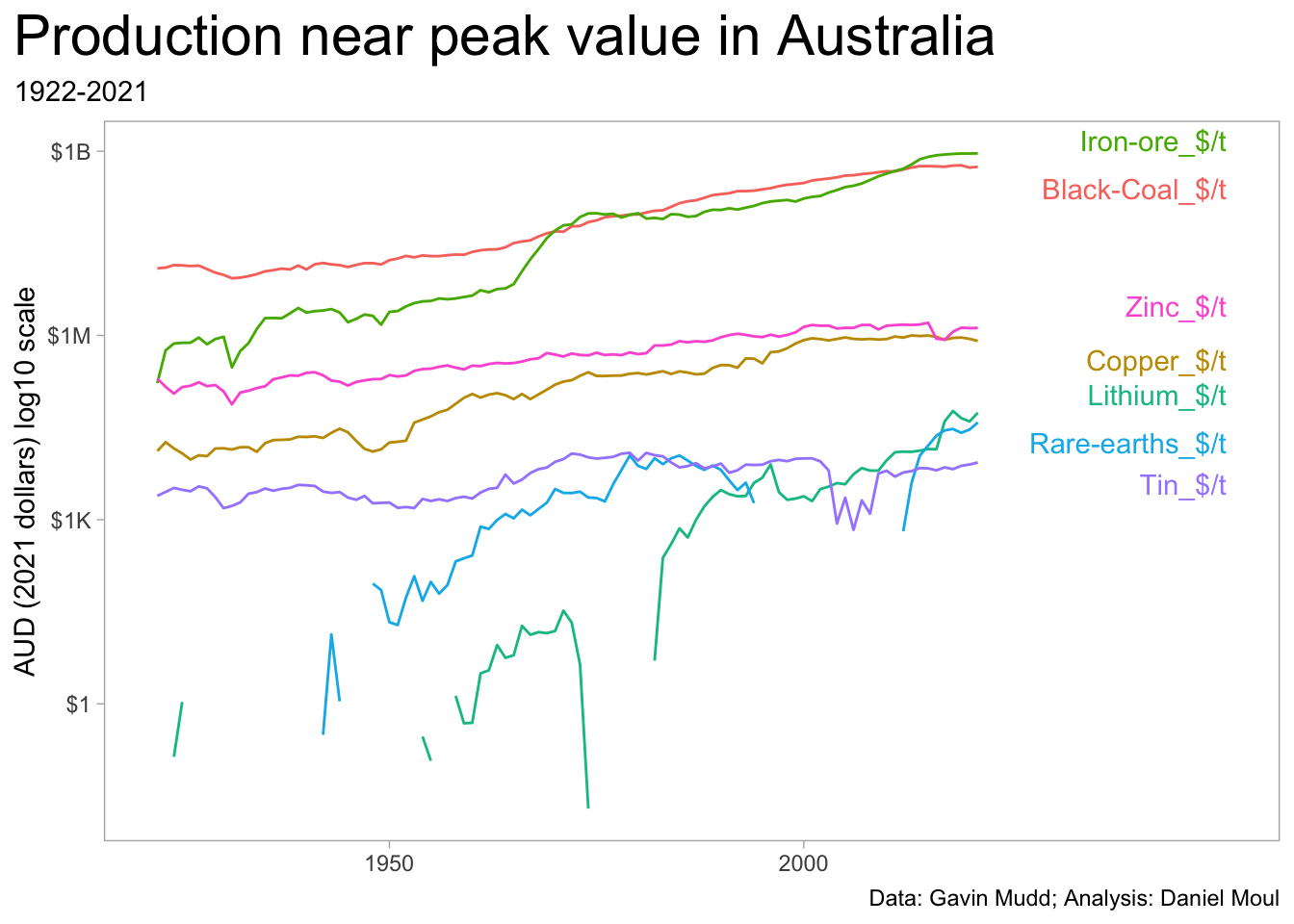
Commodities at or near peak value of production
For the following, the value of production in 2021 was within 10% of historical peak value.
Show the code
<- dta_yearly_long |> filter (year == max (year, na.rm = TRUE ) & value_2021_pct_of_max >= peak_production_cutoff) <- dta_yearly_long |> inner_join (peak_products %>% select (product_price),by = "product_price" )<- data_for_plot |> filter (! is.na (mass)) |> mutate (final_year = max (year),.by = product_price) |> filter (year == max (year),.by = product_price)|> ggplot (aes (year, mass, color = product_price, group = product_price)) + geom_line (na.rm = TRUE , show.legend = FALSE ) + geom_text_repel (data = labels_for_plot,aes (max (year) + 30 , mass, label = product_price),hjust = 1 , vjust = 0.5 , show.legend = FALSE , direction = "y" , force = 0.4 ) + scale_x_continuous (breaks = c (1850 , 1900 , 1950 , 2000 )) + scale_y_log10 (labels = label_number (scale_cut = cut_short_scale (),prefix = "$" ),+ labs (title = glue ("Production near peak value in Australia" ),subtitle = glue ("{year_first}-{year_last}" ),x = NULL ,y = "AUD (2021 dollars) log10 scale" ,caption = my_caption
Table
Show the code
|> filter (year == 2021 ) |> select (product_name, units_price, value_2021, value_max_2021) |> mutate (value_pct_of_max = value_2021 / value_max_2021) |> arrange (desc (value_2021), desc (value_pct_of_max)) |> mutate (cum_pct = cumsum (value_2021 / sum (value_2021, na.rm = TRUE )),rowid = row_number ()) |> gt () |> tab_header (md ("**Australian mining value extracted 2021**<br>*Australian dollars (AUD)*" )) |> fmt_currency (columns = c (value_2021, value_max_2021),decimals = 0 ,currency = "AUD" ,suffixing = TRUE ) |> fmt_percent (columns = c (value_pct_of_max, cum_pct),decimals = 0 ) |> sub_missing () |> tab_source_note (md ("*Data: Gavin Mudd. Analysis: Daniel Moul*" ))
Table 3.1: Australian mining value extracted in 2021
Australian mining value extracted 2021 Australian dollars (AUD)
product_name
units_price
value_2021
value_max_2021
value_pct_of_max
cum_pct
rowid
Iron-ore
$/t
$164B
$164B
100%
50%
1 Black-Coal
$/t
$97B
$101B
96%
80%
2 Gold
$/kg
$24B
$27B
88%
88%
3 Copper
$/t
$10B
$10B
100%
91%
4 Alumina
$/t
$7B
$10B
72%
93%
5 Zinc
$/t
$5B
$6B
91%
94%
6 Nickel
$/t
$4B
$7B
51%
96%
7 Bauxite
$/t
$4B
$4B
87%
97%
8 Lithium
$/t
$3B
$3B
100%
98%
9 Rare-earths
$/t
$2B
$2B
100%
98%
10 Lead
$/t
$1B
$2B
71%
98%
11 Silver
$/kg
$1B
$2B
76%
99%
12 Manganese
$/t
$1B
$6B
23%
99%
13 Uranium
$/t
$384M
$1B
37%
99%
14 Cobalt
$/t
$380M
$503M
75%
100%
15 Tin
$/t
$377M
$377M
100%
100%
16 Synthetic-rutile
$/t
$238M
$490M
49%
100%
17 Diamonds
$/carat
$230M
$926M
25%
100%
18 Garnet
$/t
$140M
$399M
35%
100%
19 Ilmenite
$/t
$127M
$206M
62%
100%
20 Rutile
$/t
$123M
$303M
40%
100%
21 Antimony
$/t
$58M
$73M
78%
100%
22 Phosphate-rock
$/t
$44M
$317M
14%
100%
23 Tantalum
$/t
$24M
$441M
5%
100%
24 Leucoxene
$/t
$22M
$32M
68%
100%
25 Tungsten
$/t
$3M
$56M
5%
100%
26 Chromium
$/t
—
$1B
—
—
27 Graphite
$/t
—
$3M
—
—
28 Molybdenum
$/t
—
$3M
—
—
29 Monazite
$/t
—
$10M
—
—
30
Data: Gavin Mudd. Analysis: Daniel Moul