9 Dams, waterways, and watersheds

Almost all dams are associated with a waterway.¹ A dam is either the origin of a waterway, or a break in its flow.

Show the code

dams_and_rivers <- dams_no_geo |>
  filter(
    str_detect(riverName, "^[A-Za-z]"), #get rid of mostly junk
    riverName != "unknnown"
  ) |>
  mutate(water_name = str_to_lower(riverName)) |>
  filter(
    !str_detect(
      water_name,
      c("unknown|unknnown|unnamed|na|n[/]a|0|^u[/]n |^un |u[/]s")
    ),
    # !str_detect(water_name, c("off( )?([-])?stream|([-])?( )?os|os-|off([ -]( ?))?channel|off |^os |none|^u[/]n |^un "))
    !str_detect(
      water_name,
      c(
        "off( )?([-])?stream|([-])?( )?os|os-|off([ -]( ?))?channel|off |^os |none|^u[/]n |^un "
      )
    )
  ) |>
  mutate(
    water_name = str_remove(
      water_name,
      "^ut to |^unt of |^unt of unt of |^unk of "
    ),
    water_name = str_replace(
      water_name,
      "(.+)(-( )?tr$| trib$)",
      "tributary to \\1"
    ),
    water_name = str_replace_all(
      water_name,
      c(
        "[/]" = " / ",
        "[.]" = ". ",
        "\\(" = " ",
        "\\)" = " ",
        '"' = "",
        #"[-]" = "- ",
        " ck[.] | ck " = " creek ",
        " crk[.]| crk" = " creek",
        " cr([.])?$| ck$" = " creek",
        "( )?riv$" = " river",
        "rvr" = "river",
        "( r|r[.])( )?$" = " river",
        "bch|br[.| ]|br[-]|br$" = "branch ",
        "^trib([.])? " = "tributary ",
        "fk" = "fork",
        "(t)?tr to( )?" = "tributary to ",
        "tr[.-]( )?" = "tributary to ",
        "tr (of )?" = "tributary to ",
        "tri (to)?" = "tributary to ",
        ", trib( |[.]|[/])" = " tributary to ",
        "trib[.]([-])?" = " tributary to ",
        "trib (of|to)?" = " tributary to ",
        "trib[/]" = " tributary to ",
        "trib[-]" = " tributary to ",
        "tributary( )[-]" = "tributary to",
        "tributary to - " = "tributary to ",
        "tributary of" = "tributary to",
        "to to|to of" = "to",
        "n[.]f[.]" = "north fork ",
        "e[.]f[.]" = "east fork ",
        "s[.]f[.]" = "south fork ",
        "w[.]f[.]" = "west fork ",
        "^e([.])? " = "east ",
        "^e[.]| e[.]" = " east ",
        " e[.]" = " east ",
        "^w([.])? " = "west ",
        "^w[.]| w[.]" = " west ",
        " w " = " west ",
        "^n([.])? |^no([.])? " = "north ",
        "^n[.]| n[.]" = " north ",
        " n " = " north ",
        "nork |noth " = "north ",
        "^s[.]| s[.]" = " south ",
        " s " = " south ",
        " so[.]" = " south ",
        "^s([.])? |^so([.])? " = "south ",
        "no[.]([ ]+)? fork" = "north fork"
      ),
    ),
    trib_to = str_extract(
      water_name,
      "(?<=tributary (of|to )?).+|(?= tributary).+"
    ),
    trib_to = str_remove_all(trib_to, "to |^ ")
  ) |>
  mutate(
    water_name = str_remove(
      water_name,
      ", trib to$|^tr-( )?|[-]( )?tr|[-][ ]+?tr"
    ),
    water_name = str_replace_all(
      water_name,
      c(
        "badriver" = "bad river",
        "tobad river" = "bad river",
        "trimissouri" = "tributary to missouri"
      )
    ),
    water_name = str_squish(water_name),
    water_name_root = str_remove(water_name, "tributary (to )?")
  ) |>
  mutate(
    water_type = case_when(
      str_detect(water_name, "fork|prong|branch") ~ "fork",
      str_detect(water_name, "tributary") ~ "tributary",
      str_detect(water_name, "creek|brook| bk$|draw") ~ "creek",
      str_detect(water_name, "race|drain") ~ "race",
      str_detect(water_name, "arroyo|gulch|coulee|draw$") ~ "arroyo",
      .default = "river"
    ),
    water_type = factor(
      water_type,
      levels = c("river", "fork", "tributary", "creek", "race", "arroyo")
    )
  ) |>
  filter(str_detect(water_name, "^[A-Za-z]")) |> # get rid of more mostly junk after removing some prefixes
  select(
    water_name,
    water_type,
    trib_to,
    water_name_root,
    riverName,
    name,
    nidId,
    state,
    nidStorage,
    yearCompleted,
    starts_with("is_")
  )

9.1 Types of waterways associated with dams

Show the code

dams_and_rivers_count_by_state <- dams_and_rivers |>
  count(water_name, water_type, water_name_root, state, sort = TRUE) |>
  arrange(state, water_name_root)

dams_and_rivers_count_by_state_simplified <- dams_and_rivers |>
  count(water_type, state, sort = TRUE) |>
  arrange(state)

dams_and_rivers_for_plotting <-
  left_join(
    dams,
    left_join(
      dams_and_rivers_count_by_state |>
        select(-n),
      dams_and_rivers |>
        select(nidId, state, water_name, water_name_root, riverName, starts_with("is_")),
      by = join_by(state, water_name, water_name_root)
    ),
    by = join_by(nidId, state, riverName)
    )


###### Bad river watershed
#  https://www.usgs.gov/national-hydrography/access-national-hydrography-products
# # The Bad River HUC8 code
# bad_river_huc8 <- "10140102"
# Manually downloaded from https://prd-tnm.s3.amazonaws.com/index.html?prefix=StagedProducts/Hydrography/NHD/HU8/Shape/

bad_river_watershed <- st_read(here("data/raw/usgs/NHD-10140102/NHD_H_10140102_HU8_Shape/Shape"),
                        quiet = TRUE)

bad_river_watershed_with_buffer <- st_buffer(bad_river_watershed, 
                                             dist = watershed_buffer) # in meters

dams_in_buffer_bbox <- st_bbox(bad_river_watershed_with_buffer)

# using mask() on a spatVector does better than st_join(join = st_within)
dams_in_bad_river_watershed_tmp <-
  st_crop(dams_and_rivers_for_plotting, bad_river_watershed) |>
  st_join(st_as_sf(st_union(bad_river_watershed)), 
          join = st_within, left = FALSE) |>
   mutate(water_type = case_when(
    str_detect(water_name, "fork")      ~ "fork",
    str_detect(water_name, "tributary") ~ "tributary",
    .default =                            "tributary"
  ),
  water_type = factor(water_type, levels = c("river", "fork", "tributary")),
  primary_owner = fct_collapse(primaryOwnerTypeId ,"State and Local" = c("State", "Local Government"))) 
  
# using mask() on a spatVector does better than st_join(join = st_within)
dams_in_bad_river_watershed <- mask(crop(vect(dams_in_bad_river_watershed_tmp), bad_river_watershed), 
                                               vect(bad_river_watershed)) |>
  st_as_sf()

dams_in_buffer_around_bad_river_watershed_tmp <-
  st_crop(dams_and_rivers_for_plotting, bad_river_watershed_with_buffer) |>
  st_join(st_as_sf(st_union(bad_river_watershed_with_buffer)) |>
                     st_make_valid(), 
          join = st_within, left = FALSE) |>
  st_filter(st_union(dams_in_bad_river_watershed), 
            .predicate = st_disjoint) |> # anti_join()
   mutate(water_type = case_when(
    str_detect(water_name, "fork")      ~ "fork",
    str_detect(water_name, "tributary") ~ "tributary",
    .default =                            "river"
  ),
  water_type = factor(water_type, levels = c("river", "fork", "tributary")),
  primary_owner = fct_collapse(primaryOwnerTypeId ,"State and Local" = c("State", "Local Government"))) 

# using mask() on a spatVector does better than st_join(join = st_within)
dams_in_buffer_around_bad_river_watershed <- mask(crop(vect(dams_in_buffer_around_bad_river_watershed_tmp), 
                                                                  bad_river_watershed_with_buffer), 
                                               vect(bad_river_watershed),
                                               inverse = TRUE) |>
  st_as_sf()

# TEST
# ggplot() +
#   geom_sf(data = bad_river_watershed |>
#             st_union(),
#           color = muted("firebrick"),
#           width = 0.2,
#           alpha = 0.3) +
#   geom_sf(data = dams_in_bad_river_watershed,
#           color = "firebrick", fill = NA) +
#  geom_sf(data = dams_in_buffer_around_bad_river_watershed,
#           color = "darkblue") +
#   labs(
#     title = "Dams in and near the Bad River watershed",
#     subtitle = "TEST: there shouldn't be any blue markers in the watershed",
#     x = NULL,
#     y = NULL,
#     caption = my_caption
#   )

###### Get OSM data

sd_bad_river_osm_fname <- here("data/processed/st-bad-river-osm.rds")
sd_bad_river_osm_points_fname <- here("data/processed/st-bad-river-osm-points.rds")
sd_bad_river_roads_fname <- here("data/processed/st-bad-river-osm-roads.rds")
sd_bad_river_places_fname <- here("data/processed/st-bad-river-osm-places.rds")
sd_bad_river_dams_osm_fname <- here("data/processed/st-bad-river-dams-osm.rds")

### River lines and points (points include additional tributary detail)

# Features from https://wiki.openstreetmap.org/wiki/Map_features#Water
# requires osmdata package

if(!file.exists(sd_bad_river_osm_fname) | !file.exists(sd_bad_river_osm_points_fname)) {
  
  sd_bad_river_list <- dams_in_buffer_bbox |> # includes buffer around Bad River watershed
    opq()%>%
    add_osm_feature(key = "waterway",
                    value = c("river", "stream")) %>%
    osmdata_sf()
  
  sd_bad_river_points <- sd_bad_river_list$osm_points |> 
    st_transform(crs = "NAD83") # |>
    # st_crop(dams_in_buffer_bbox) # not needed (bbox used in initial query)
  
  write_rds(sd_bad_river_points, sd_bad_river_osm_points_fname)
  
  sd_bad_river <- sd_bad_river_list$osm_multilines |> # multilines are best for "clean" map
    filter(str_detect(name, "Bad River")) |>
    st_transform(crs = "NAD83") # |>
    # st_crop(dams_in_buffer_bbox) # not needed (bbox used in initial query)
  
  write_rds(sd_bad_river, sd_bad_river_osm_fname)
  
  
} else {
  
  sd_bad_river <- read_rds(sd_bad_river_osm_fname)
  sd_bad_river_points <- read_rds(sd_bad_river_osm_points_fname)
  
}

### Roads

# Features from https://wiki.openstreetmap.org/wiki/Map_features#Water
# requires osmdata package

if(!file.exists(sd_bad_river_roads_fname)) {
  
  sd_bad_roads_list <- dams_in_buffer_bbox |> # includes buffer around Bad River watershed
    opq()%>%
    add_osm_feature(key = "highway",
                    value = c("motorway", "trunk", "primary", "secondary", "tertiary", "unclassified", "road",
                              "track")) %>%
    osmdata_sf()
  
  # sd_bad_river_road_points <- sd_bad_roads_list$osm_points |> 
  #   st_transform(crs = "NAD83") # |>
  #   # st_crop(dams_in_buffer_bbox) # not needed (bbox used in initial query)
  # 
  # # write_rds(sd_bad_river_road_points, sd_bad_river_osm_road_points_fname)
  
  sd_bad_river_roads <- sd_bad_roads_list$osm_lines |> # multilines are best for "clean" map
    # filter(str_detect(name, "Bad River")) |>
    st_transform(crs = "NAD83") |>
    # st_zm() |> # get rid of error:
    #            # Problem while converting geom to grob.
    #            # ℹ Error occurred in the 2nd layer.
    #            # Caused by error in `check.length()`:
    #            # ! 'gpar' element 'fontsize' must not be length 0
    st_crop(dams_in_buffer_bbox) |> # perhaps not needed (bbox used in initial query)?
    remove_empty(which = "cols") |>
    select(osm_id, name, NHS, expressway, highway, ref, surface, geometry) |>
    mutate(length = st_length(geometry),
           length_m = as.numeric(length),
           length_mi = length_m * 0.6213712)
  
  write_rds(sd_bad_river_roads, sd_bad_river_roads_fname)
  
  
} else {
  
  sd_bad_river_roads <- read_rds(sd_bad_river_roads_fname)
  # sd_bad_river_road_points <- read_rds(sd_bad_river_osm_points_fname)
  
}


### Places: cities, towns, etc.

# Features from https://wiki.openstreetmap.org/wiki/Map_features#Water
# requires osmdata package

if(!file.exists(sd_bad_river_places_fname)) {
  
  sd_bad_river_places_list <- dams_in_buffer_bbox |> # includes buffer around Bad River watershed
    opq()%>%
    add_osm_feature(key = "place",
                    value = c("city", "town", "village", "hamlet")) %>%
    osmdata_sf()
  
  # sd_bad_river_road_points <- sd_bad_roads_list$osm_points |> 
  #   st_transform(crs = "NAD83") # |>
  #   # st_crop(dams_in_buffer_bbox) # not needed (bbox used in initial query)
  # 
  # # write_rds(sd_bad_river_road_points, sd_bad_river_osm_road_points_fname)
  
  sd_bad_river_places <- sd_bad_river_places_list$osm_points |> # not many polygons or multipolygons
    # filter(str_detect(name, "Bad River")) |>
    st_transform(crs = "NAD83") |>
    # st_zm() |> # get rid of error:
    #            # Problem while converting geom to grob.
    #            # ℹ Error occurred in the 2nd layer.
    #            # Caused by error in `check.length()`:
    #            # ! 'gpar' element 'fontsize' must not be length 0
    st_crop(dams_in_buffer_bbox) |> # perhaps not needed (bbox used in initial query)?
    remove_empty(which = "cols") |>
    select(osm_id, name, place, population, geometry)
  
  write_rds(sd_bad_river_places, sd_bad_river_places_fname)
  
  
} else {
  
  sd_bad_river_places <- read_rds(sd_bad_river_places_fname)
  # sd_bad_river_road_points <- read_rds(sd_bad_river_osm_points_fname)
  
}


### Dam points
# Each Dam in OSM has a NID reference

# if(!file.exists(sd_bad_river_dams_osm_fname)) {
#   
#   sd_dams_osm <- dams_in_buffer_bbox |> # includes buffer around Bad River watershed
#     opq()%>%
#     add_osm_feature(key = "waterway",
#                     value = c("dam")) %>%
#     osmdata_sf()
#   
#   sd_dams_osm_points <- sd_dams_osm$osm_points |>
#     st_transform(crs = "NAD83") |>
#     filter(!is.na(name)) # |>
#     # st_crop(dams_in_buffer_bbox) # not needed (bbox used in initial query)
#   
#   write_rds(sd_dams_osm_points, sd_bad_river_dams_osm_fname)
#   
# } else {
#   
#   sd_dams_osm_points <- read_rds(sd_bad_river_dams_osm_fname)
#   
# }

# dam_intersect_watershed <- 
#   inner_join(
#     dams_in_bad_river_watershed |>
#       st_drop_geometry(),
#     sd_dams_osm_points |>
#       mutate(name = str_remove(name, " Dam$")),
#     by = join_by(nidId == `ref:US:NID`) #, name)
#   ) |>
#   st_as_sf(crs = "NAD83") |>
#   remove_empty(which = "cols") |>
#   remove_constant()
# 
# dam_intersect_buffer <- 
#   inner_join(
#     dams_in_buffer_around_bad_river_watershed |>
#       st_drop_geometry(),
#     sd_dams_osm_points |>
#       mutate(name = str_remove(name, " Dam$")),
#     by = join_by(nidId == `ref:US:NID`) #, name)
#   ) |>
#   st_as_sf(crs = "NAD83") |>
#   remove_empty(which = "cols") |>
#   remove_constant()


###### Detailed stream, river and lake/reservoir data from National Hydrology Dataset (NHD)

# sd1_layers not needed once we know which layers to load
# sd1_layers <- st_layers(here("data/raw/usgs/NHD-SD/NHD_H_South_Dakota_State_GDB.zip"))

sd_flowline_fname <- here("data/processed/sd_flowline.rds")
sd_waterbody_fname <- here("data/processed/sd_waterbody.rds")

if(!file.exists(sd_flowline_fname)) {
  
  sd_NHDFlowLine <-  st_read(here("data/raw/usgs/NHD-SD/NHD_H_South_Dakota_State_GDB.zip"),
                             layer = "NHDFlowLine",
                             quiet = TRUE) |>
    clean_names() |>
    remove_empty(which = "cols") |>
    remove_constant() |>
    st_zm(drop = TRUE) |> # don't need elevation
    st_transform("NAD83") |>
    st_crop(dams_in_buffer_bbox)
  
  write_rds(sd_NHDFlowLine, sd_flowline_fname)
  
} else {
  
  sd_NHDFlowLine <- read_rds(sd_flowline_fname)
}

if(!file.exists(sd_waterbody_fname)) {
  
  sd_NHDWaterbody <-  st_read(here("data/raw/usgs/NHD-SD/NHD_H_South_Dakota_State_GDB.zip"),
                              layer = "NHDWaterbody",
                              quiet = TRUE) |>
    clean_names() |>
    remove_empty(which = "cols") |>
    remove_constant() |>
    filter(ftype %in% c(390, 436)) |> 
    st_zm(drop = TRUE) |> # don't need elevation
    st_transform("NAD83") |>
    st_crop(dams_in_buffer_bbox)
  
  write_rds(sd_NHDWaterbody, sd_waterbody_fname)
  
} else {
  
  sd_NHDWaterbody <- read_rds(sd_waterbody_fname)
}

# Note: ftype: 390: LakePond, 436: Reservoir as per https://www.usgs.gov/ngp-standards-and-specifications/national-hydrography-dataset-nhd-data-dictionary-feature-classes

## Now subset

sd_NHDFlowLine_bad_river <- sd_NHDFlowLine |>
  filter(str_detect(gnis_name, "Bad River"))

# TODO: delete the following
# bad_river_bbox <- dams_in_buffer_bbox 

# TODO: Get rid of superfluous variables
                          
# dta_flowline_for_plot <- sd_NHDFlowLine |> # TODO: Don't need to do this st_crop() (was already done above)
#   st_crop(dams_in_buffer_bbox)

sd_NHDFlowLine_missouri_river <- sd_NHDFlowLine |>
  filter(str_detect(gnis_name, "Missouri River"))

# sd_NHDWaterbody_near_bad_river <- sd_NHDWaterbody

bad_river_length_km <- sd_NHDFlowLine_bad_river |>
  filter(gnis_name == "Bad River") |> # omit forks
  pull(lengthkm) |>
  sum() 

bad_river_length_mi <- bad_river_length_km * 0.621371

There are many names for small waterways, and they are not always used consistently–unsurprising given that naming happened independently over hundreds of years by many people and in the wide variety of geographical environments. In the NID we find the following (after significant data cleaning):

Show the code

dams_and_rivers |>
  count(water_type, sort = TRUE) |>
  mutate(pct = n / sum(n)) |>
  adorn_totals(where = "row") |>
  gt() |>
  tab_header(md(glue("**Types of waterways associated with dams<br>in the NID**"))) |>
  tab_options(table.font.size = 11) |>
  cols_align(columns = water_type,
             align = "left"
  ) |>
  fmt_number(columns = "n",
             decimals = 0
  ) |>
fmt_percent(columns = "pct",
             decimals = 0
  )

Table 9.1

Types of waterways associated with dams in the NID
water_type	n	pct
tributary	30,662	46%
creek	19,339	29%
fork	8,612	13%
river	7,314	11%
arroyo	524	1%
race	40	0%
Total	66,491	100%

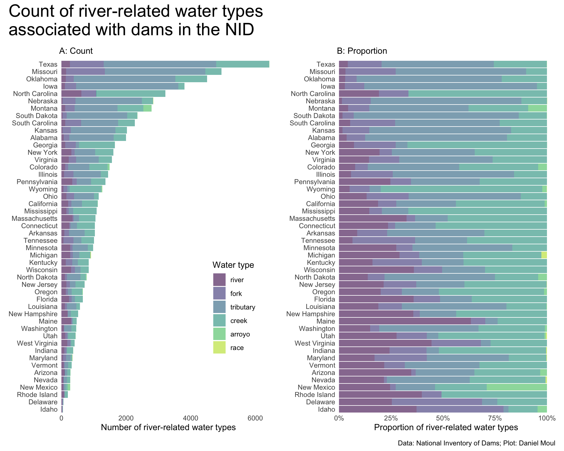
Looking at the counts and proportions of these terms by state in Figure 9.1.

North Carolina, Georgia, and Wyoming have the most usages of “creek”.
It’s not surprising that historically Spanish-speaking areas have the most use of “arroyo” (New Mexico and Arizona). I’m surprised to see so many uses of “arroyo” in North Dakota, Idaho, and Wyoming.
“Race” seems to be a peculiarity of Michigan with only a small additional number in Indiana, Utah, and Nevada.

Show the code

dta_for_plot <- dams_and_rivers_count_by_state_simplified |>
  mutate(state = fct_reorder(state, n, sum),
         water_type = factor(water_type, levels = rev(c("river", "fork", "tributary", "creek", "arroyo", "race")))
         )
  
p1 <- dta_for_plot |> 
  ggplot() +
  geom_col(aes(n, state, fill = water_type)) +
  scale_x_continuous(expand = expansion(mult = c(0.01, 0.04))) +
  scale_fill_viridis_d(end = 0.9,
                       direction = -1) +
  guides(fill = guide_legend(position = "inside",
                             reverse = TRUE)) +
  theme(legend.position.inside = c(0.8, 0.3)) +
  labs(
    subtitle = "A: Count",
    x = "Number of river-related water types",
    y = NULL,
    fill = "Water type"
  )

p2 <-  dta_for_plot |>
  ggplot() +
  geom_col(aes(n, state, fill = water_type),
           position = "fill",
           show.legend = FALSE) +
  scale_x_continuous(expand = expansion(mult = c(0.01, 0.04)),
                     labels = label_percent()) +
  scale_fill_viridis_d(end = 0.9,
                       direction = -1) +
  labs(
    subtitle = "B: Proportion",
    x = "Proportion of river-related water types",
    y = NULL,
    fill = "Water type"
  )

p1 + p2 + 
  plot_annotation(
    title = "Count of river-related water types\nassociated with dams in the NID",
    caption = my_caption,
  )

9.2 Case study: watershed of the Bad River South Dakota

The bad river watershed is located in southwest South Dakota just north of the famous Badlands and Badland National Park. It’s a dry environment. Nonetheless, there are a lot of dams within its watershed.

Show the code

dams_in_bad_river_watershed |>
  st_drop_geometry() |>
  count(water_type, sort = TRUE) |>
  mutate(pct = n / sum(n)) |>
  adorn_totals(where = "row") |>
  gt() |>
  tab_header(md(glue("**Types of waterways associated with dams<br>in the Bad River watershed**"))) |>
  tab_options(table.font.size = 11) |>
  cols_align(columns = water_type,
             align = "left"
  ) |>
  fmt_number(columns = "n",
             decimals = 0
  ) |>
fmt_percent(columns = "pct",
             decimals = 0
  )

Table 9.2

Types of waterways associated with dams in the Bad River watershed
water_type	n	pct
tributary	388	96%
fork	16	4%
Total	404	100%

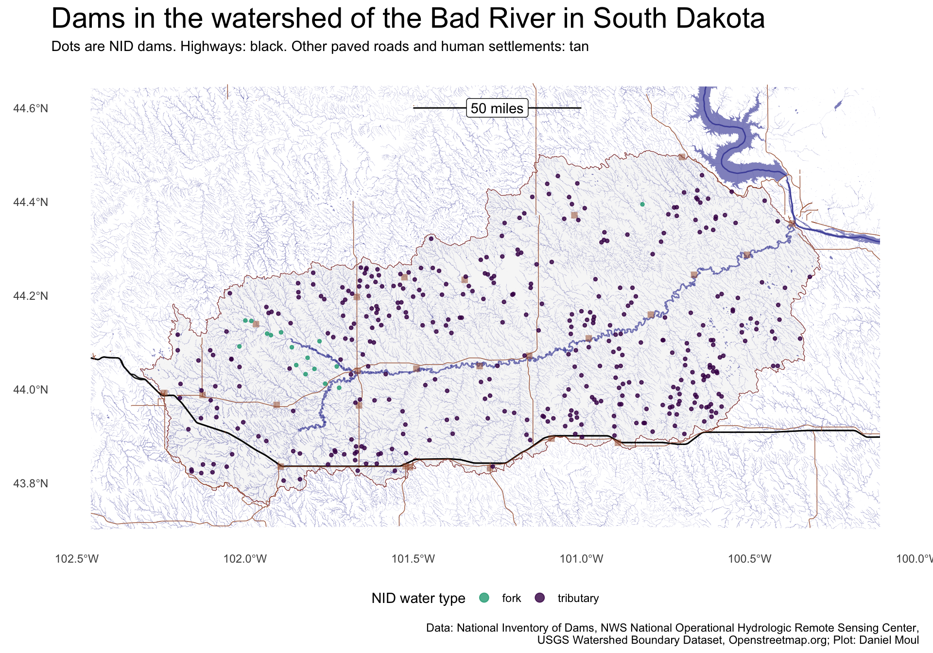
The Bad River flows north-east-east into the Missouri River at Fort Pierre. Across from it, on the east side of the Missouri, is Pierre, the state capital.

Show the code

# TODO: The following works, but I would prefer a 10-mile length bar on the plot (not 49.7 mi)

### what is the East-West distance in miles of 0.5 degree at 44.0 degrees?
p1 <- st_point(c(-101, 44.6)) #44.4
p2 <- st_point(c(-101.5, 44.6)) #44.4

# https://en.wikipedia.org/wiki/Longitude
# https://en.wikipedia.org/wiki/Earth_radius
# r_earth = 6371 # km
# dist_long = (pi / 180) * r_earth * cos(44 * pi / 180)
# 79.98694 km = 49.7 mi
# TODO: Use the above to try out a 10 mi bar

myline <- st_sfc(list(p1, p2)) |>
  st_set_crs("WGS84") |>
  st_transform("NAD83")

linestring <- st_combine(st_sfc(list(p1, p2))) %>% st_cast("LINESTRING") |>
  st_set_crs("WGS84") |>
  st_transform("NAD83")

linestring_mi_label <- drop_units(st_length(linestring)) * 0.000621371

myline_df <- st_as_sf(linestring) |>
  st_set_crs("WGS84") |>
  st_transform("NAD83")

# Now the label
p1 <- st_point(c(-101, 44.6))
p2 <- st_point(c(-101.5, 44.6))
p3 <- st_point(c(-102, 44.6))
myline <- st_sfc(list(p1, p2, p3)) |>
  st_set_crs("WGS84") |>
  st_transform("NAD83")
linestring <- st_combine(st_sfc(list(p1, p2))) %>% st_cast("LINESTRING") |>
  st_set_crs("WGS84") |>
  st_transform("NAD83")

myline_df_label <- st_as_sf(linestring) |>
  st_set_crs("WGS84") |>
  st_transform("NAD83") |>
  mutate(center = st_centroid(x),
         name = "50 miles")

st_geometry(myline_df_label) <- myline_df_label$center

distance_bar <- st_as_sf(
  st_union(
    myline_df, 
    myline_df_label
  )
)

Most dams are associated with “tributary” waterways; the exceptions are near the north and south forks.

Show the code

dams_in_bad_river_watershed |>
  ggplot() +
  geom_sf(data = bad_river_watershed |>
            st_union() |>
            st_crop(dams_in_buffer_bbox),
          color = muted("firebrick"),
          linewidth = 0.2,
          alpha = 0.3) +
  geom_sf(data = sd_NHDFlowLine, # many small streams
          color = "darkblue",# "grey60",
          linewidth = 0.05,
          alpha = 0.3) +
  geom_sf(data = sd_bad_river, # the main river
          # size = 0.01,
          linewidth = 0.5,
          color = "darkblue", # "grey70",
          alpha = 0.5) +
  geom_sf(data = sd_NHDFlowLine_missouri_river, # the bigger river that Bad River flows into
          # size = 0.01,
          # linewidth = 0.5,
          color = "darkblue", # "grey70",
          alpha = 0.5) +
   geom_sf(data = sd_NHDWaterbody, # the lake just upriver from where Bad River enters the Missouri
          # size = 0.01,
          linewidth = 1,
          color = NA, #"darkblue", # "grey70",
          fill = "darkblue",
          alpha = 0.5) +
  # roads
  geom_sf(data = sd_bad_river_roads |> # roads in the buffer bbox
            filter(highway == "motorway") |>
            st_crop(st_union(sd_NHDWaterbody)),
          linewidth = 0.5,
          color = "black", #"darkblue", # "grey70",
          fill = NA,
          alpha = 0.9) +
  geom_sf(data = sd_bad_river_roads |> # roads in the buffer bbox
            filter(highway %in% c("primary", "secondary") |
                     highway == "tertiary" & surface %in% c("paved", "asphalt", "concrete")
                   ) |>
            st_crop(st_union(sd_NHDWaterbody)),
          linewidth = 0.25,
          color = "sienna", 
          fill = NA,
          alpha = 0.9) +
  # places
  geom_sf(data = sd_bad_river_places |> # places in the buffer bbox
            filter(!is.na(place)) |>
            st_join(st_as_sf(st_union(bad_river_watershed)), 
                    join = st_within, left = FALSE),
          size = 2, # was 0.15
          color = "sienna", 
          # fill = "gold",
          shape = 15, # solid square 
          alpha = 0.5) +  
  geom_sf(aes(color = water_type),
          size = 1,  # The NID dataset points
          alpha = 0.8
  ) +
  geom_sf(data = distance_bar) + # distance bar line
  geom_sf_label(data = distance_bar,
                aes(label = name)) + # distance bar label
  scale_color_viridis_d(end = 0.60,
                        direction = -1) +
  guides(color = guide_legend(override.aes = list(size = 3))) +
  theme(legend.position = "bottom") +
  labs(
    title = "Dams in the watershed of the Bad River in South Dakota",
    subtitle = glue("Dots are NID dams. Highways: black. Other paved roads and human settlements: tan"),
    x = NULL,
    y = NULL,
    color = "NID water type",
    caption = my_caption_nid_nws_wbd_oms
  )

Figure 9.2: Dams in the watershed of the Bad River in South Dakota

Show the code

## Not in the watershed

dta_for_plot <- dams_in_buffer_around_bad_river_watershed |>
  filter(water_name_root == "bad river")

n_dams_in_error <- nrow(dta_for_plot)

dta_for_plot |>
  ggplot() +
  geom_sf(data = bad_river_watershed |>
            st_union() |>
            st_crop(dams_in_buffer_bbox),
          color = muted("firebrick"),
          linewidth = 0.2,
          alpha = 0.3) +
  geom_sf(data = sd_NHDFlowLine, # many small streams
          color = "darkblue",# "grey60",
          linewidth = 0.05,
          alpha = 0.3) +
  geom_sf(data = sd_bad_river, # the main river
          # size = 0.01,
          linewidth = 0.5,
          color = "darkblue", # "grey70",
          alpha = 0.5) +
  geom_sf(data = sd_NHDFlowLine_missouri_river, # the bigger river that Bad River flows into
          # size = 0.01,
          linewidth = 0.5,
          color = "darkblue", # "grey70",
          alpha = 0.5) +
   geom_sf(data = sd_NHDWaterbody, # the lake just upriver from where Bad River enters the Missouri
          # size = 0.01,
          linewidth = 1,
          color = NA, #"darkblue", # "grey70",
          fill = "darkblue",
          alpha = 0.5) +
  geom_sf(aes(color = water_type),
          size = 2,  # The NID dataset points
          alpha = 0.8
          ) +
  geom_sf(data = distance_bar) + # distance bar line
  geom_sf_label(data = distance_bar,
                aes(label = name)) + # distance bar label
  scale_color_viridis_d(end = 0.60,
                        direction = -1) +
  guides(color = guide_legend(override.aes = list(size = 3))) +
  theme(legend.position = "bottom") +
  labs(
    title = glue("There are {n_dams_in_error} dams associated with the Bad River\nbut are not in its watershed"),
    subtitle = "Two are debatable (on the boundary of the watershed). The other two seem to be recorded in error.",
    x = NULL,
    y = NULL,
    color = "NID water type",
    caption = my_caption_nid_nws_wbd_oms
  )

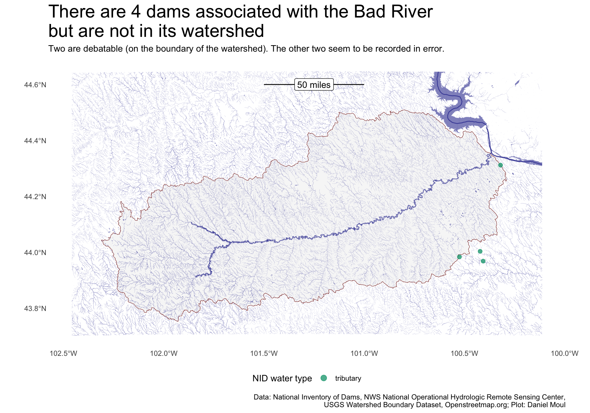
Figure 9.3: Dams associated with the Bad River but not in its the watershed

Show the code

ggplot() +
  geom_sf(data = bad_river_watershed |>
            st_union() |>
            st_crop(dams_in_buffer_bbox),
          color = muted("firebrick"),
          linewidth = 0.2,
          alpha = 0.3) +
  geom_sf(data = sd_bad_river_points |>
            st_crop(dams_in_buffer_bbox), 
          size = 0.005,
          color = "grey90",
          alpha = 0.05) +
  geom_sf(data = sd_bad_river,
          size = 0.005,
          color = "grey70",
          alpha = 0.05) + # was 0.3
  geom_sf(data = dams_in_bad_river_watershed |>
            filter(primary_owner == "Private"), 
          size = 1,
          alpha = 0.2
          ) + 
  geom_sf(data = dams_in_bad_river_watershed |>
            filter(primary_owner != "Private"), 
          aes(color = primary_owner),
          size = 1,
          alpha = 0.8
          ) + 
  scale_color_viridis_d(end = 0.6,
                       direction = -1) +
  guides(color = guide_legend(override.aes = list(size = 3))) +
  theme(legend.position = "bottom") +
  labs(
    title = "Publically-owned dams\nare not on the main river",
    subtitle = glue("Federal dams are owned by the US Forest Service.\nBad River watershed South Dakota"),
    color = "Primary owner",
    caption = my_caption_nid_nws_wbd_oms
  )

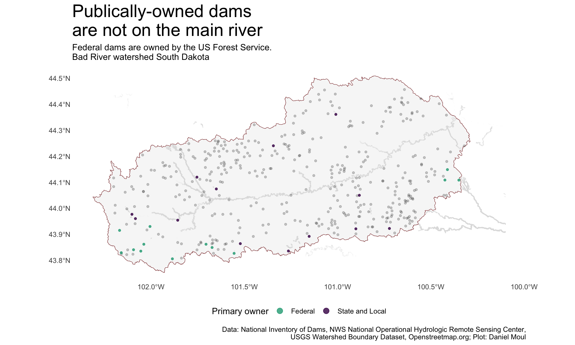
Figure 9.4: Publically owned dams are not on the main river

Show the code

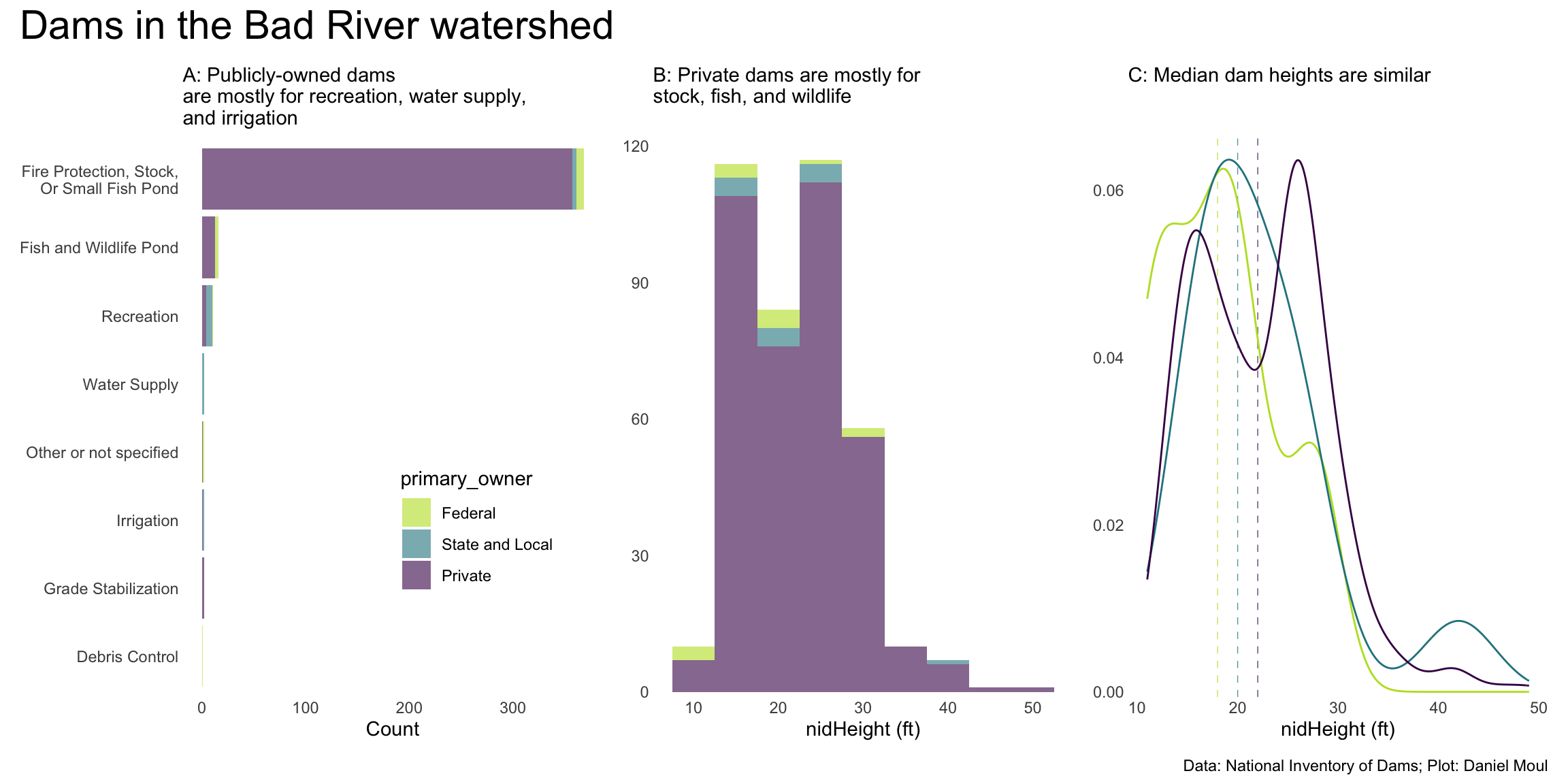
median_nidHeight_by_owner <- dams_in_bad_river_watershed |>
  st_drop_geometry() |>
  summarize(median_nidHeight = median(nidHeight, na.rm = TRUE),
         .by = primary_owner)

p1 <- dams_in_bad_river_watershed |>
  count(primary_owner, primaryPurposeId) |>
  mutate(primaryPurposeId = fct_reorder(primaryPurposeId, n, sum)) |> 
  ggplot(aes(n, primaryPurposeId, fill = primary_owner)) +
  geom_col() +
  scale_x_continuous(labels = label_number(scale_cut = cut_short_scale())) +
  scale_fill_viridis_d(end = 0.90,
                       direction = -1) +
  scale_color_viridis_d(end = 0.90,
                       direction = -1) +
  guides(fill = guide_legend(position = "inside")) +
  theme(legend.position.inside = c(0.7, 0.3)) +
  labs(
    subtitle = glue("A: Publicly-owned dams",
                    "\nare mostly for recreation, water supply,", 
                    "\nand irrigation"), 
    x = "Count",
    y = NULL
  )

p2 <- dams_in_bad_river_watershed |>
  ggplot(aes(nidHeight, fill = primary_owner)) +
  geom_histogram(binwidth = 5,
                 alpha = 0.6) +
  scale_x_continuous(labels = label_number(scale_cut = cut_short_scale())) +
  scale_y_continuous(expand = expansion(mult = c(0.01, 0.04))) +
  scale_fill_viridis_d(end = 0.90,
                       direction = -1) +
  scale_color_viridis_d(end = 0.90,
                       direction = -1) +
  guides(color = "none",
         fill = "none") +
  labs(
    subtitle = glue("B: Private dams are mostly for", 
                    "\nstock, fish, and wildlife"),
    x = "nidHeight (ft)",
    y = NULL
  )

p3 <- dams_in_bad_river_watershed |>
  ggplot(aes(nidHeight, color = primary_owner)) +
  geom_vline(data = median_nidHeight_by_owner,
             aes(xintercept = median_nidHeight, color = primary_owner),
             lty = 2,
             linewidth = 0.25,
             alpha = 0.75) +
  geom_density() +
  scale_x_continuous(labels = label_number(scale_cut = cut_short_scale())) +
  scale_y_continuous(expand = expansion(mult = c(0.01, 0.04))) +
  scale_color_viridis_d(end = 0.90,
                       direction = -1) +
  guides(color = "none",
         fill = "none") +
  labs(
    subtitle = glue("C: Median dam heights are similar"),
    x = "nidHeight (ft)",
    y = NULL
  )

p1 + p2 + p3 +
  plot_annotation(
    title = "Dams in the Bad River watershed",
    caption = my_caption
  )

Figure 9.5: Dams on the Bad River and tributaries

The exceptions are dams for tailings and other waste products like coal ash, which are designed not to allow the contents behind the dam to flow.↩︎