3 Modeling and model comparison
As noted in the EDA section:
The relationship between \(log_{10}(pop\_density)\) and \(log_{10}(light\_avg)\) in figures 2.4 and 2.5) isn’t quite linear, and there are differences by state. So I expect simple linear models to perform worse than more sophisticated ones. Nonetheless, I want to see how good linear models are, since they are simple and inexpensive.
In this section I do the following:
- Prepare train-test and holdout data sets
- Build (and where necessary, train) some models, then compare them using performance metrics
- Test the best performing models against the holdout data set.
I use the following performance metrics:
- Concordance correlation coefficient (ccc) according the help for
yardstick::ccc()“is a metric of both consistency/correlation and accuracy,” - R-Squared. I use
yardstick::rsq()which according to the documentation “is simply the squared correlation between truth and estimate … [that] guarantees a value on \((0,1)\).”
I use metrics that are scale-free, since I want the freedom to use models with different transformations of the data. The principle metric is ccc.
# For 2000
data_df <- tar_read(all_df) %>%
  #fix NAs
  mutate(atotal = if_else(!is.na(atotal), atotal, calc_area),
         pop_density_official = if_else(!is.na(pop_density_official), pop_density_official, pop_density)) %>%
  # drop a small number of data errors/artifacts
  filter(light_avg > 1e-5)
# prepare data for train-test and holdout
d_df <- data_df %>%
# dplyr::select(state:pop_density_official) %>%
# avoid zero values
mutate(log_light_avg = log10(light_avg + 1e-6),
log_pop_density = log10(pop_density + 1e-6),
log_pop_density_official = log10(pop_density_official + 1e-6)) %>%
select(state, county, light_avg, log_light_avg, pop_density, log_pop_density, pop_density_official, log_pop_density_official)
# following https://cran.r-project.org/web/packages/rsample/vignettes/Working_with_rsets.html
set.seed(123)
main_split = initial_split(d_df, strata = c("state"))
train_split <- analysis(main_split)
holdout <- assessment(main_split)
light_folds <- vfold_cv(train_split, v = n_folds, repeats = 1)# For 2010
data_df_c <- tar_read(all_df_c) %>%
#fix NAs
mutate(atotal = if_else(!is.na(atotal), atotal, calc_area),
pop_density_official = if_else(!is.na(pop_density_official), pop_density_official, pop_density)) %>%
# drop a small number of data errors/artifacts
filter(light_avg > 1e-5)# prepare data for train-test and holdout
assess_df <- data_df_c %>%
# dplyr::select(state:pop_density_official) %>%
# avoid zero values
mutate(log_light_avg = log10(light_avg + 1e-6),
log_pop_density = log10(pop_density + 1e-6),
log_pop_density_official = log10(pop_density_official + 1e-6)) %>%
select(state, county, light_avg, log_light_avg, pop_density, log_pop_density, pop_density_official, log_pop_density_official)
set.seed(2021)# inspiration/source: Dave Robinson's coding videos; see https://github.com/dgrtwo/data-screencasts
prep_juice <- function(x) juice(prep(x))
mset <- metric_set(rsq, ccc) # use scale-free metrics (not rmse)
grid_control <- control_grid(save_pred = TRUE,
save_workflow = TRUE,
extract = extract_model)
augment.workflow <- function(x, newdata, ...) {
predict(x, newdata, ...) %>%
bind_cols(newdata)
}
predict_on_holdout <- function(workflow, tbl_train, tbl_test) {
workflow %>%
fit(tbl_train) %>%
augment(tbl_test)
}
# for use in fit_resamples()
keep_pred <- control_resamples(save_pred = TRUE, save_workflow = TRUE)3.1 Train and test on training data set
3.1.1 lin1: pop_density ~ light_avg
Let’s start simple. In lin1 the data is concentrated in smaller radiance values, and the model is depressing the slope of the line due to outliers at high pop_density.
lm_model <-
  linear_reg() %>%
  set_engine("lm") %>%
  set_mode("regression")

my_formula <- "pop_density ~ light_avg"

lin_rec <- recipe(
  data = analysis(light_folds$splits[[1]]),
  formula =  as.formula(my_formula))

lin1_wf <-
  workflow() %>%
  add_recipe(lin_rec) %>%
  add_model(lm_model)

lin1_res <- lin1_wf %>%
  fit_resamples(resamples = light_folds,
                metrics = mset,
                control = keep_pred)

lin1_metric_summary <- lin1_res %>%
  collect_metrics() %>%
  mutate(model = glue("lin1: {my_formula}")) %>%
  dplyr::select(".metric", .estimate = "mean", "n", "std_err", "model")

metric_summary_for_plot <- glue("{lin1_metric_summary[[1, 1]]} = {round(lin1_metric_summary[[1, 2]], 3)}",
                       "; {lin1_metric_summary[[2, 1]]} = {round(lin1_metric_summary[[2, 2]], 3)}")

lin1_res %>%
  collect_predictions() %>%
  ggplot(aes(x = pop_density, y = .pred)) +
  geom_abline(lty = 2, alpha = 0.5) +
  geom_point(alpha = 0.15) +
  labs(title = glue("{lin1_metric_summary$model}"),
       subtitle = glue("Actual and predicted pop_density: {metric_summary_for_plot}")
  )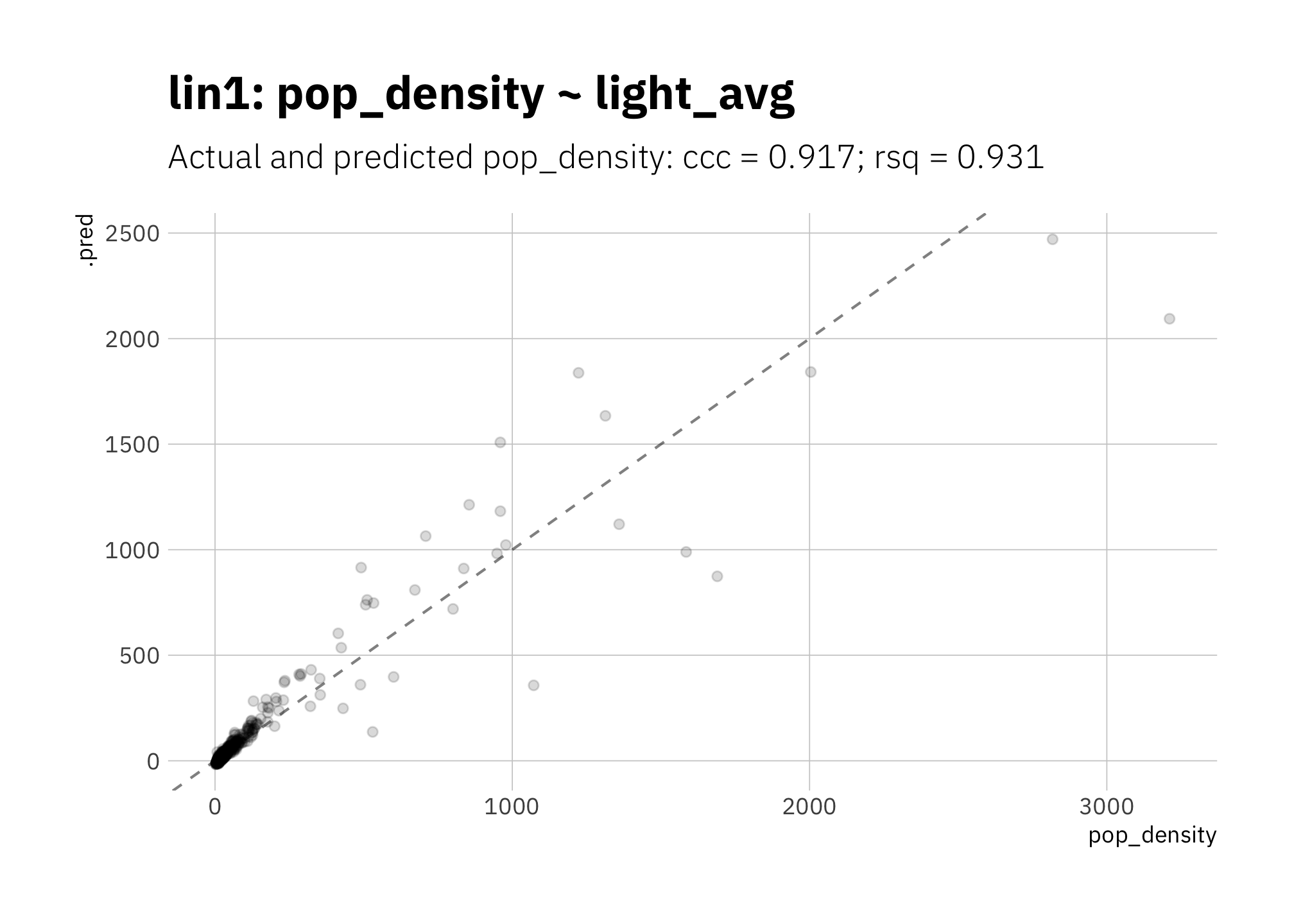
Figure 3.1: lin1: Simplest linear model
3.1.2 lin2: pop_density_official ~ light_avg
Should I use official area values from the US Census Bureau to calculate population density instead of area values calculated based on the county boundaries? In a word: no. Using official area values, rsq and ccc are slightly lower than lin 1 (figure 3.1), perhaps because pop_density is calculated using the same boundaries I’m using to determine which light pixels are part of each county, and therefore I’m dealing with similar error in both. I use the area values I calculated in all other models.
my_formula <- "pop_density_official ~ light_avg"

lin_rec2 <- recipe(
  data = analysis(light_folds$splits[[1]]),
  formula =  as.formula(my_formula))

lin2_wf <-
  workflow() %>%
  add_recipe(lin_rec2) %>%
  add_model(lm_model) # defined above

lin2_res <- lin2_wf %>%
  fit_resamples(resamples = light_folds,
                metrics = mset,
                control = keep_pred)

lin2_metric_summary <- lin2_res %>%
  collect_metrics() %>%
  mutate(model = glue("lin2: {my_formula}")) %>%
  dplyr::select(".metric", .estimate = "mean", "n", "std_err", "model")

metric_summary_for_plot <- glue("{lin2_metric_summary[[1, 1]]} = {round(lin2_metric_summary[[1, 2]], 3)}",
                       "; {lin2_metric_summary[[2, 1]]} = {round(lin2_metric_summary[[2, 2]], 3)}")

lin2_res %>%
  collect_predictions() %>%
  ggplot(aes(x = pop_density_official, y = .pred)) +
  geom_abline(lty = 2, alpha = 0.5) +
  geom_point(alpha = 0.15) +
  labs(title = glue("{lin2_metric_summary$model}"),
       subtitle = glue("Actual and predicted pop_density_official: {metric_summary_for_plot}")
  )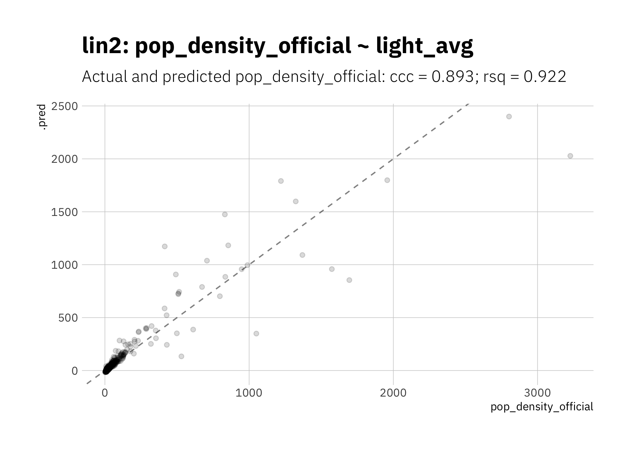
Figure 3.2: lin2: Using official area values to calculate population density
3.1.3 lin3: log_pop_density ~ log_light_avg
With both predictor and response on a log scale, performance metrics are better. Compare with lin1 in Figure 3.1.
my_formula <- "log_pop_density ~ log_light_avg"

lin_rec3 <- recipe(
  data = analysis(light_folds$splits[[1]]),
  formula =  as.formula(my_formula))

lin3_wf <-
  workflow() %>%
  add_recipe(lin_rec3) %>%
  add_model(lm_model) # defined above

lin3_res <- lin3_wf %>%
  fit_resamples(resamples = light_folds,
                metrics = mset,
                control = keep_pred)

lin3_metric_summary <- lin3_res %>%
  collect_metrics() %>%
  mutate(model = glue("lin3: {my_formula}")) %>%
  dplyr::select(".metric", .estimate = "mean", "n", "std_err", "model")

metric_summary_for_plot <- glue("{lin3_metric_summary[[1, 1]]} = {round(lin3_metric_summary[[1, 2]], 3)}",
                       "; {lin3_metric_summary[[2, 1]]} = {round(lin3_metric_summary[[2, 2]], 3)}")

lin3_res %>%
  collect_predictions() %>%
  ggplot(aes(x = log_pop_density, y = .pred)) +
  geom_abline(lty = 2, alpha = 0.5) +
  geom_point(alpha = 0.15) +
  # coord_obs_pred() +
  labs(title = glue("{lin3_metric_summary$model}"),
       subtitle = glue("Actual and predicted log_pop_density: {metric_summary_for_plot}")
  )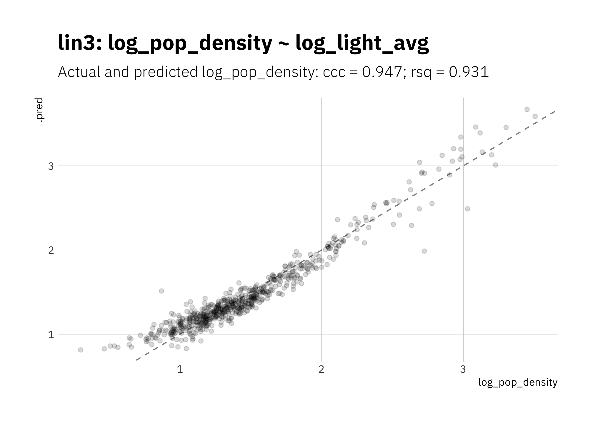
Figure 3.3: lin3: Simplest linear model with log10 transformations
3.1.4 pol1: log_light_avg ~ poly(log_pop_density, 2)
Since the data in Figure 2.4 looks like it has close to a quadratic relationship (a convex curve), let’s try a second order polynomial. Performance is quite good.
my_formula_basic <- "log_pop_density ~ log_light_avg"
my_formula <- "log_pop_density ~ poly(log_light_avg, 2)"

pol1_rec <- recipe(
  data = analysis(light_folds$splits[[1]]),
  formula =  as.formula(my_formula_basic)) %>%
  step_poly(log_light_avg, degree = 2)

pol1_wf <-
  workflow() %>%
  add_recipe(pol1_rec) %>%
  add_model(lm_model) # defined above

pol1_res <- pol1_wf %>%
  fit_resamples(resamples = light_folds,
                metrics = mset,
                control = keep_pred)

pol1_metric_summary <- pol1_res %>%
  collect_metrics() %>%
  mutate(model = glue("pol1: {my_formula}"))  %>%
  dplyr::select(".metric", .estimate = "mean", "n", "std_err", "model")

metric_summary_for_plot <- glue("{pol1_metric_summary[[1, 1]]} = {round(pol1_metric_summary[[1, 2]], 3)}",
                       "; {pol1_metric_summary[[2, 1]]} = {round(pol1_metric_summary[[2, 2]], 3)}")

pol1_res %>%
  collect_predictions() %>%
  ggplot(aes(x = log_pop_density, y = .pred)) +
  geom_abline(lty = 2, alpha = 0.5) +
  geom_point(alpha = 0.15) +
  labs(title = glue("{pol1_metric_summary$model}"),
       subtitle = glue("Actual and predicted log_pop_density: {metric_summary_for_plot}")
  )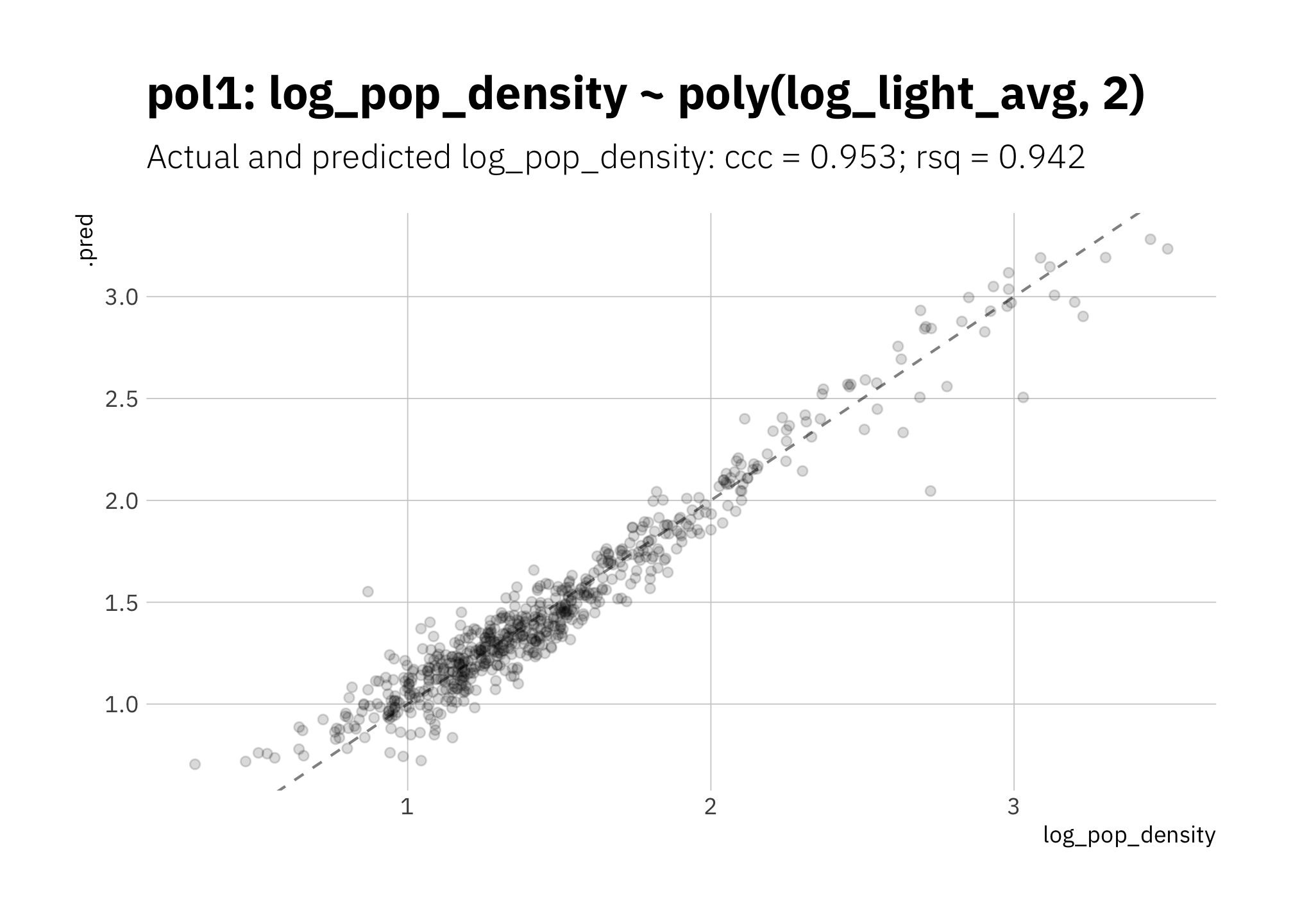
Figure 3.4: pol1: Linear model with second order polynomial
3.1.5 lme1: multi-level model with lme4::lmer
Since states differ in the range and distribution of radiance values, are there improvements if I use a fixed effects model “log_pop_density ~ log_light_avg + (log_light_avg | state)?” Unfortunately not. There is no meaningful improvement over Figure 3.3. Apparently state doesn’t hold enough unique information to be helpful.
lme_model <-
  linear_reg() %>%
  set_engine("lmer") %>%
  set_mode("regression")

my_formula <- "log_pop_density ~ log_light_avg + (log_light_avg | state)"

lme1_wf <-
  workflow() %>%
  add_variables(outcomes = log_pop_density,
                predictors = c(log_light_avg, state)
                ) %>%
  add_model(
    lme_model,
    formula = as.formula(my_formula)
    )

lme1_res <- lme1_wf %>%
  fit_resamples(resamples = light_folds,
                metrics = mset,
                control = keep_pred)

lme1_metric_summary <- lme1_res %>%
  collect_metrics() %>%
  mutate(model = glue("lme1: {my_formula}")) %>%
  dplyr::select(".metric", .estimate = "mean", "n", "std_err", "model")

metric_summary_for_plot <- glue("{lme1_metric_summary[[1, 1]]} = {round(lme1_metric_summary[[1, 2]], 3)}",
                                "; {lme1_metric_summary[[2, 1]]} = {round(lme1_metric_summary[[2, 2]], 3)}")

lme1_res %>%
  collect_predictions() %>%
  ggplot(aes(x = log_pop_density, y = .pred)) +
  geom_abline(lty = 2, alpha = 0.5) +
  geom_point(alpha = 0.15) +
  theme(plot.title = element_text(size = 14)) +
  labs(title = glue("{lme1_metric_summary$model}"),
       subtitle = glue("Actual and predicted log_pop_density: {metric_summary_for_plot}")
  )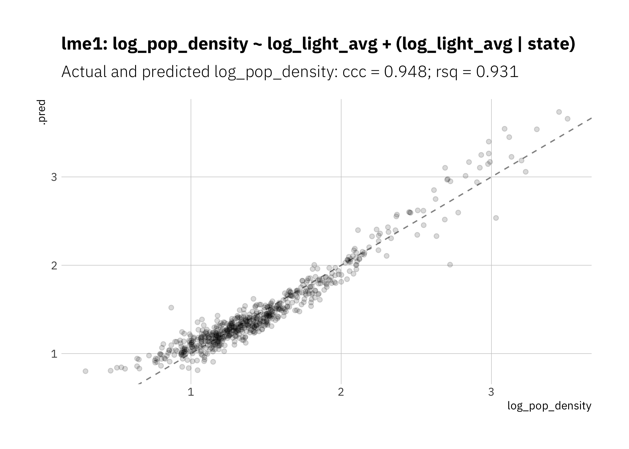
Figure 3.5: lme1: Multi-level model using ‘state’
3.1.6 bs1: linear model with b-spline
Since lin3 (figure 3.3) seems to be overestimating high and low radiance, let’s try a spline. First I tune the model to determine how many knots to include in the spline:
bs_rec <- recipe(log_pop_density ~ log_light_avg,
                  data = analysis(light_folds$splits[[1]])) %>%
  step_ns(log_light_avg, deg_free = tune("log_light_avg"))

bs_model <-
  linear_reg() %>%
  set_engine("lm") %>%
  set_mode("regression")

my_formula = "log_pop_density ~ bs(log_light_avg)"

bs1_wf <-
  workflow() %>%
  add_recipe(bs_rec) %>%
  add_model(bs_model)

k_grid <- tibble(log_light_avg = 1:6)

bs_tune <- bs1_wf %>%
  tune_grid(resamples = light_folds,
            grid = k_grid,
            metrics = mset,
control = grid_control)autoplot(bs_tune) +
labs(title = "Tuning bs1")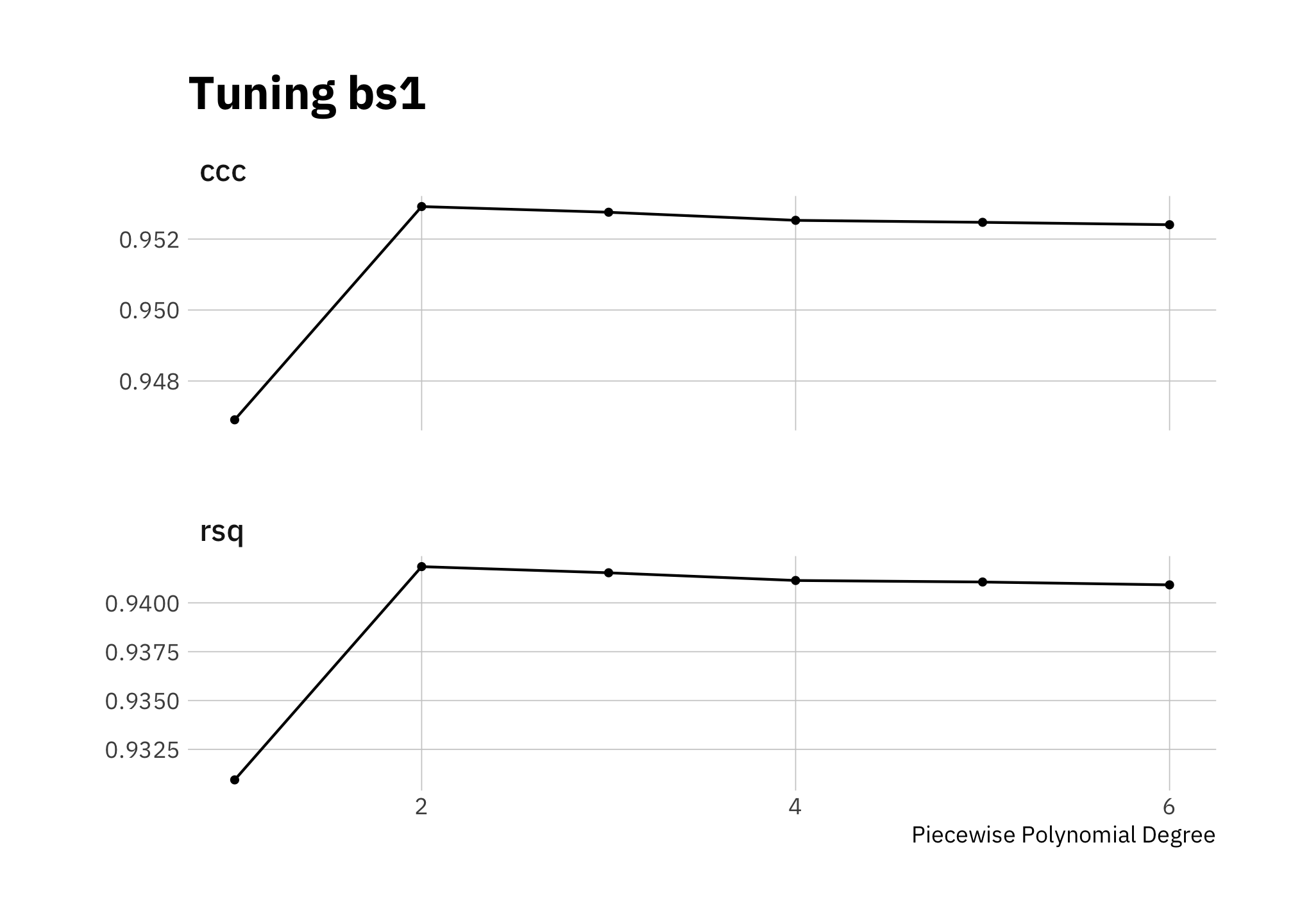
Figure 3.6: Tuning bs1
I’ll use 2 knots, which maximizes both ccc and rsq.
bs_wf_best <- bs1_wf %>%
  finalize_workflow(select_best(bs_tune, metric = "ccc"))

select_best(bs_tune, metric = "ccc") %>%
gt()| log_light_avg | .config |
|---|---|
| 2 | Preprocessor2_Model1 |
Both ccc and rsq are slightly better than lin3, and the high and low predictions are not consistently overestimated:
bs1_res <- bs_wf_best %>%
  fit_resamples(resamples = light_folds,
                metrics = mset,
                control = keep_pred)

bs1_metric_summary <- bs1_res %>% collect_metrics() %>%
  mutate(model = glue("bs1: {my_formula}")) %>%
  dplyr::select(".metric", .estimate = "mean", "n", "std_err", "model")

metric_summary_for_plot <- glue("{bs1_metric_summary[[1, 1]]} = {round(bs1_metric_summary[[1, 2]], 3)}",
                                "; {bs1_metric_summary[[2, 1]]} = {round(bs1_metric_summary[[2, 2]], 3)}")

bs1_res %>%
  collect_predictions() %>%
  ggplot(aes(x = log_pop_density, y = .pred)) +
  geom_abline(lty = 2, alpha = 0.5) +
  geom_point(alpha = 0.15) +
  theme(plot.title = element_text(size = 14)) +
  labs(title = glue("{bs1_metric_summary$model}"),
       subtitle = glue("Actual and predicted log_pop_density: {metric_summary_for_plot}")
  )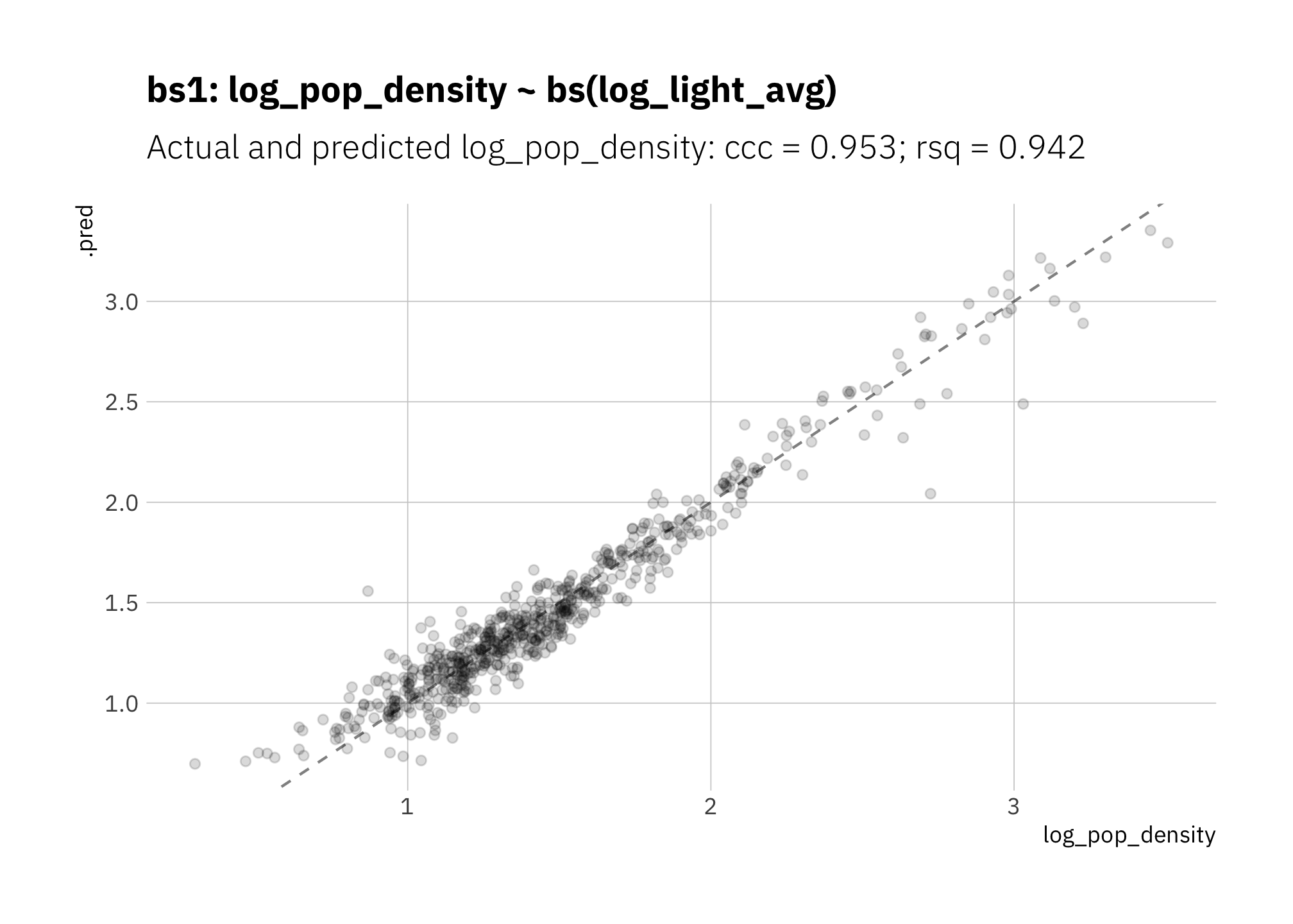
Figure 3.7: bs1: Linear model with B-spline to capture curvature
3.1.7 XGBoost: log_pop_density ~ log_light_avg + state
Now a non-linear model and one that needs training: boosted trees using XGBoost. In this model state categories are dummy variables.
set.seed(2021)

xg1_rec <- recipe(log_pop_density ~ log_light_avg + state,
                  data = analysis(light_folds$splits[[1]])) %>%
  step_dummy(state)

xg1_wf <- workflow() %>%
  add_recipe(xg1_rec) %>%
  add_model(boost_tree(mode = "regression",
                       mtry = tune(),
                       trees = tune(),
                       # tree_depth = , # default is 6
                       learn_rate = .01) %>% set_engine("xgboost"))

xg1_tune <- xg1_wf %>%
  tune_grid(light_folds,
            grid = crossing(mtry = c(2, 5, 8, 11),
                       trees = seq(50, 400, 50),
                       #threshold = c(0.01) # default is 0.01
                       ),
            metrics = mset,
            control = grid_control)
Tuning the model: results suggest using between 250 and 400 trees with nearly equal performance including 5, 8 or 11 variables at each split:
autoplot(xg1_tune) +
  labs(title = "Tuning xg1")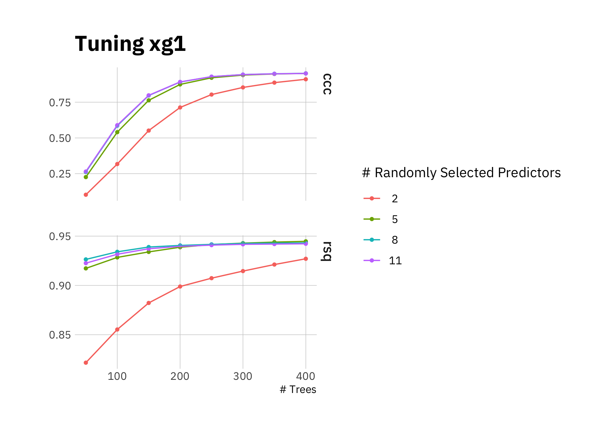
Figure 3.8: Tuning xg1
The best fit includes 400 trees and using \(mtry = 8\) to randomly sample 8 variables at each split (which is nearly all of them in this case). The benefit of 400 trees versus 300 is very small, and given we have ~650 data points for training (before considering that we are cross-validating with 10 folds), I use the lesser number. Fewer trees reduces the chance of overfitting.
xg1_wf_best <- xg1_wf %>%
  finalize_workflow(select_best(xg1_tune, metric = "ccc")) %>%
  update_model(boost_tree(mode = "regression",
                       mtry = 8,
                       trees = 300,
                       # tree_depth = 3,
                       learn_rate = .01) %>% set_engine("xgboost"))
So I use these:
print(xg1_wf_best)## ══ Workflow ═════════════════════════════════════════════════════════════════════
## Preprocessor: Recipe
## Model: boost_tree()
##
## ── Preprocessor ─────────────────────────────────────────────────────────────────
## 1 Recipe Step
##
## • step_dummy()
##
## ── Model ────────────────────────────────────────────────────────────────────────
## Boosted Tree Model Specification (regression)
##
## Main Arguments:
## mtry = 8
## trees = 300
## learn_rate = 0.01
##
## Computational engine: xgboostSummary metrics are good, however the model is underestimating most radiance values:
my_formula <- "log_pop_density ~ log_light_avg + state"

xg1_fit_best <- xg1_wf_best %>%
  fit(train_split)

xg1_res <- xg1_fit_best %>%
  last_fit(main_split, metrics = mset)

xg1_metric_summary <- xg1_res %>%
  collect_metrics() %>%
  mutate(model = glue("xg1: {my_formula}")) %>%
  mutate(n = n_folds,
         std_err = NA_real_) %>%
  dplyr::select(.metric, .estimate, n, std_err, model)

metric_summary_for_plot <- glue("{xg1_metric_summary[[2, 1]]} = {round(xg1_metric_summary[[2, 2]], 3)}",
                       "; {xg1_metric_summary[[1, 1]]} = {round(xg1_metric_summary[[1, 2]], 3)}")

xg1_res %>%
  collect_predictions() %>%
  ggplot(aes(x = log_pop_density, y = .pred)) +
  geom_abline(lty = 2, alpha = 0.5) +
  geom_point(alpha = 0.15) +
  theme(plot.title = element_text(size = 14)) +
  labs(title = glue("{xg1_metric_summary$model}"),
       subtitle = glue("Actual and predicted log_pop_density: {metric_summary_for_plot}")
  )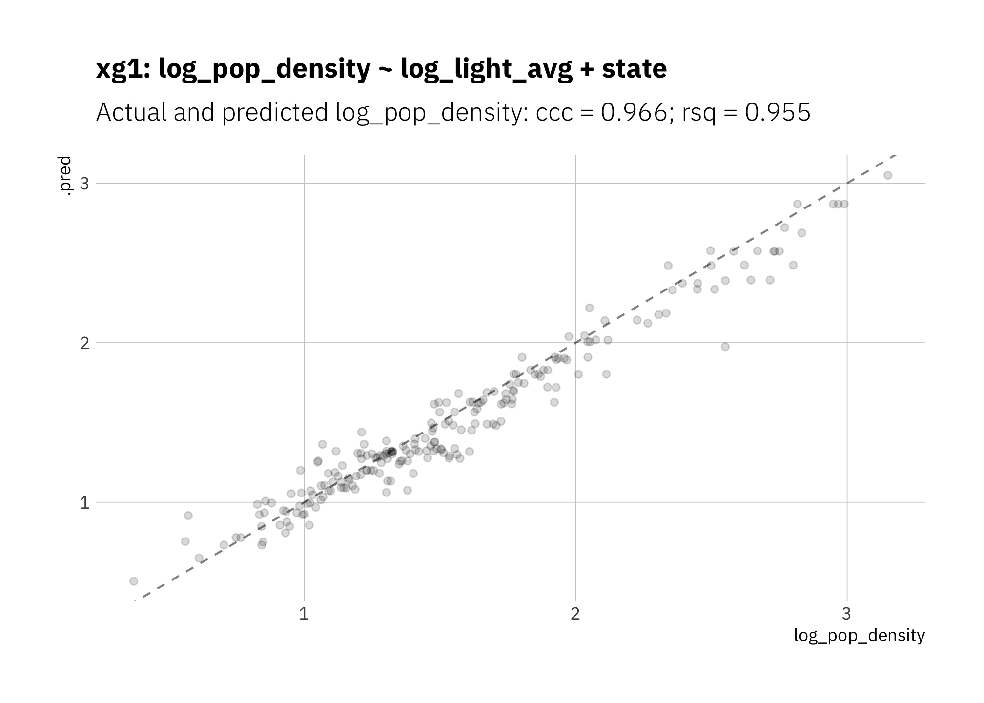
Figure 3.9: xg1: Random forest with boosted graidient descent
3.1.8 Summary of train-test results
As expected, the highest-performing model is not the simplest. lin1 and lin2 are the two worst-performing models; I exclude them from the next stage. The others (simpler and more complex) perform similarly.
all_metrics <- bind_rows(
  lin1_metric_summary,
  lin2_metric_summary,
  lin3_metric_summary,
  pol1_metric_summary,
  xg1_metric_summary,
  lme1_metric_summary,
  bs1_metric_summary,
  NULL
) %>%
  filter(.metric %in% c("ccc", "rsq"))

model_levels = all_metrics %>%
  filter(.metric == "ccc") %>%
  arrange(.estimate) %>%
  pull(model)

all_metrics %>%
  mutate(model = factor(model, levels = model_levels)) %>%
  ggplot(aes(.estimate, model)) +
  geom_errorbarh(aes(xmax = .estimate + std_err, xmin = .estimate - std_err),
                height = 0.2) +
  geom_point() +
  expand_limits(x = 1.0) +
  facet_wrap( ~ .metric, nrow = 1) +
  theme(plot.title.position = "plot") +
  labs(title = glue("Comparing model performance for metrics ",
                    "{glue_collapse(sort(unique(all_metrics$.metric)), sep = ', ')}"),
       subtitle = "Performance on train-test set",
       x = "mean metric estimate across all folds; error bars +/- std_err")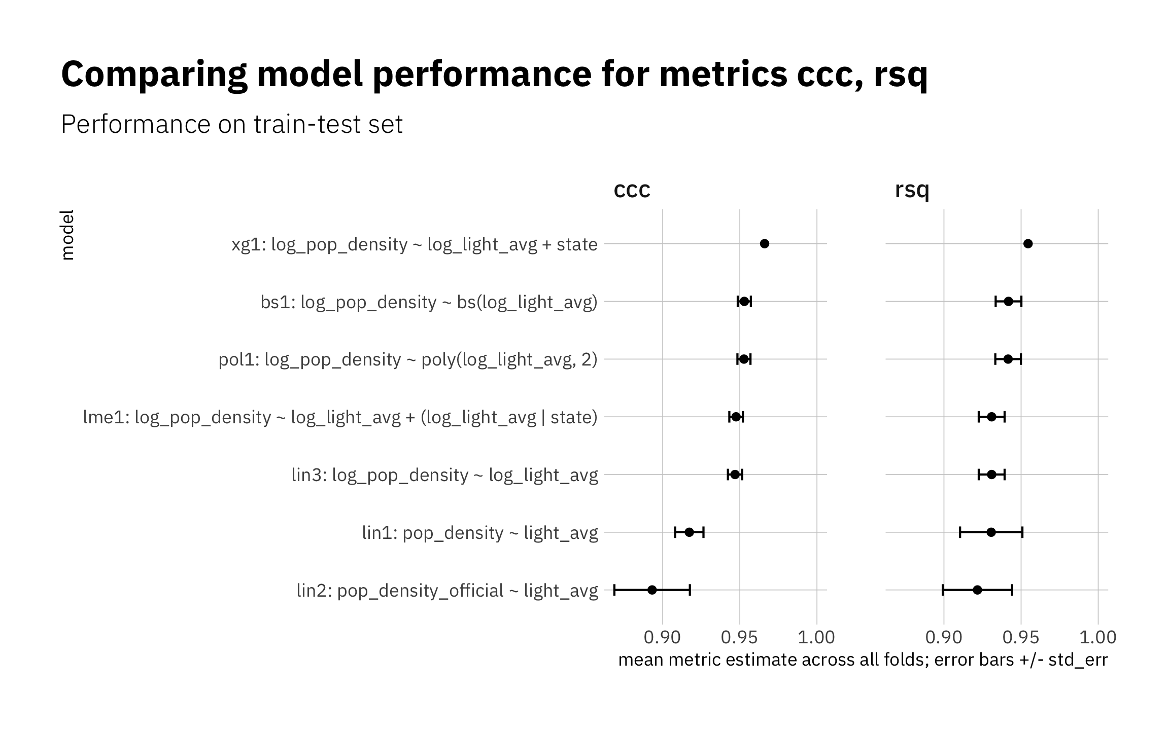
Figure 3.10: Summary of train-test results
all_metrics %>%
  arrange(.metric, desc(.estimate)) %>%
  gt() %>%
  tab_header(
    title = md("**Model evaluation on train-test data set**")
    ) %>%
  fmt_number(columns = c(.estimate, std_err),
             decimals = 3) %>%
  fmt_missing(columns = everything(),
              missing_text = "---") %>%
cols_align(columns = model, align = "left")| Model evaluation on train-test data set | ||||
|---|---|---|---|---|
| .metric | .estimate | n | std_err | model |
| ccc | 0.966 | 10 | — | xg1: log_pop_density ~ log_light_avg + state |
| ccc | 0.953 | 10 | 0.004 | bs1: log_pop_density ~ bs(log_light_avg) |
| ccc | 0.953 | 10 | 0.004 | pol1: log_pop_density ~ poly(log_light_avg, 2) |
| ccc | 0.948 | 10 | 0.004 | lme1: log_pop_density ~ log_light_avg + (log_light_avg | state) |
| ccc | 0.947 | 10 | 0.005 | lin3: log_pop_density ~ log_light_avg |
| ccc | 0.917 | 10 | 0.009 | lin1: pop_density ~ light_avg |
| ccc | 0.893 | 10 | 0.024 | lin2: pop_density_official ~ light_avg |
| rsq | 0.955 | 10 | — | xg1: log_pop_density ~ log_light_avg + state |
| rsq | 0.942 | 10 | 0.008 | bs1: log_pop_density ~ bs(log_light_avg) |
| rsq | 0.942 | 10 | 0.008 | pol1: log_pop_density ~ poly(log_light_avg, 2) |
| rsq | 0.931 | 10 | 0.008 | lin3: log_pop_density ~ log_light_avg |
| rsq | 0.931 | 10 | 0.008 | lme1: log_pop_density ~ log_light_avg + (log_light_avg | state) |
| rsq | 0.931 | 10 | 0.020 | lin1: pop_density ~ light_avg |
| rsq | 0.922 | 10 | 0.022 | lin2: pop_density_official ~ light_avg |
3.2 Assessing model performance with the holdout data set
In this section I use data the models haven’t seen yet from 2000 (the holdout data set).
lin3 summary metrics are quite good, however again the curvature in the data is visible in the way the model is overestimating high and low radiance values:
lin3_pred <- lin3_wf %>%
  predict_on_holdout(., train_split, holdout)

lin3_metric_summary <- bind_rows(
  rsq(lin3_pred, truth = log_pop_density, estimate = .pred),
  ccc(lin3_pred, truth = log_pop_density, estimate = .pred)
) %>%
  mutate(model = unique(lin3_metric_summary$model))

lin3_pred %>%
  ggplot(aes(log_pop_density, .pred, color = state)) +
  geom_abline(lty = 2, alpha = 0.5) +
  geom_point(alpha = 0.15) +
  coord_fixed() +
  labs(title = glue("{lin3_metric_summary$model}"),
       subtitle = glue("Actual and predicted log_pop_density: ",
                       "{lin3_metric_summary[[2, 1]]} = {round(lin3_metric_summary[[2, 3]], 3)}",
                       "; {lin3_metric_summary[[1, 1]]} = {round(lin3_metric_summary[[1, 3]], 3)}")
  )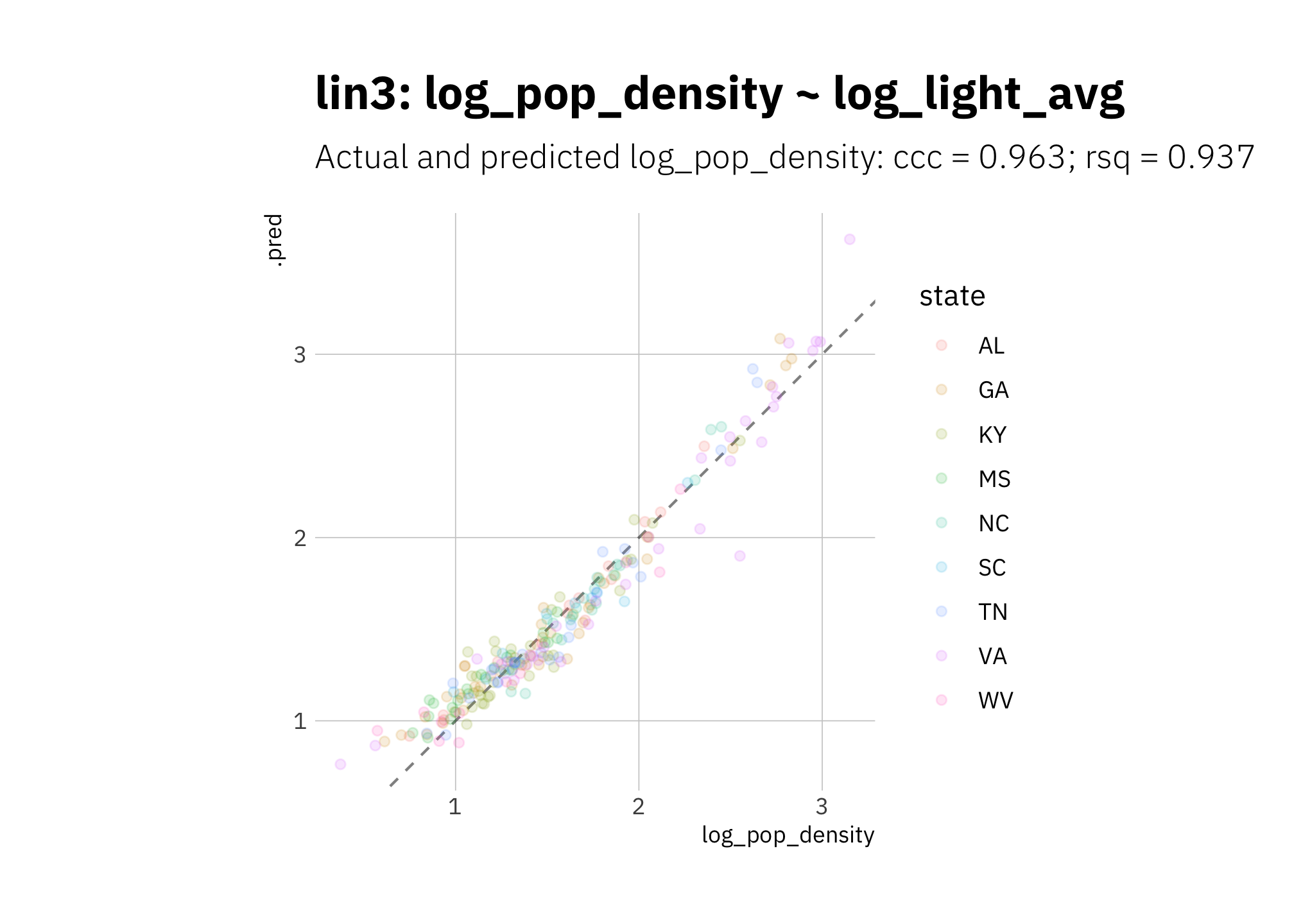
Figure 3.11: lin3 using holdout set
pol1 looks good but is slightly overestimating high radiance values:
pol1_pred <- pol1_wf %>%
  predict_on_holdout(., train_split, holdout)

pol1_metric_summary <- bind_rows(
  rsq(lin3_pred, truth = log_pop_density, estimate = .pred),
  ccc(lin3_pred, truth = log_pop_density, estimate = .pred)
) %>%
  mutate(model = unique(pol1_metric_summary$model))

pol1_pred %>%
  ggplot(aes(log_pop_density, .pred, color = state)) +
  geom_abline(lty = 2, alpha = 0.5) +
  geom_point(alpha = 0.15) +
  coord_fixed() +
  labs(title = glue("{pol1_metric_summary$model}"),
       subtitle = glue("Actual and predicted log_pop_density: ",
                       "{pol1_metric_summary[[2, 1]]} = {round(pol1_metric_summary[[2, 3]], 3)}",
                       "; {pol1_metric_summary[[1, 1]]} = {round(pol1_metric_summary[[1, 3]], 3)}")
  )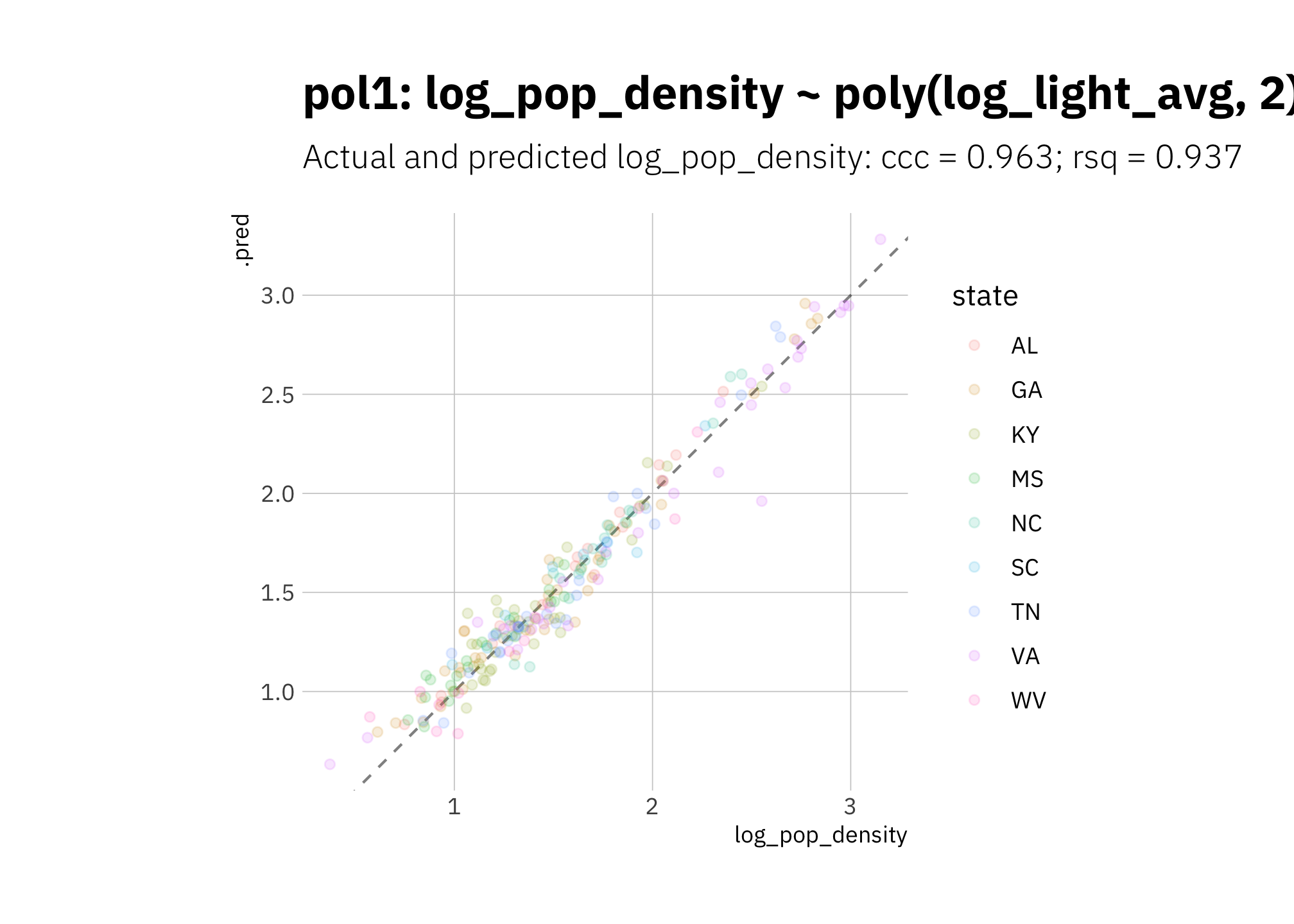
Figure 3.12: pol1 using holdout set
Again lme1 fails to do better than lin3:
# error=TRUE to continue execution in case model fails to converge

lme1_pred <- lme1_wf %>%
  predict_on_holdout(., train_split, holdout)

lme1_metric_summary <- bind_rows(
  rsq(lme1_pred, truth = log_pop_density, estimate = .pred),
  ccc(lme1_pred, truth = log_pop_density, estimate = .pred)
) %>%
  mutate(model = unique(lme1_metric_summary$model))

lme1_pred %>%
  ggplot(aes(log_pop_density, .pred, color = state)) +
  geom_abline(lty = 2, alpha = 0.5) +
  geom_point(alpha = 0.15) +
  coord_fixed() +
  labs(title = glue("{lme1_metric_summary$model}"),
       subtitle = glue("Actual and predicted log_pop_density: ",
                       "{lme1_metric_summary[[2, 1]]} = {round(lme1_metric_summary[[2, 3]], 3)}",
                       "; {lme1_metric_summary[[1, 1]]} = {round(lme1_metric_summary[[1, 3]], 3)}")
  )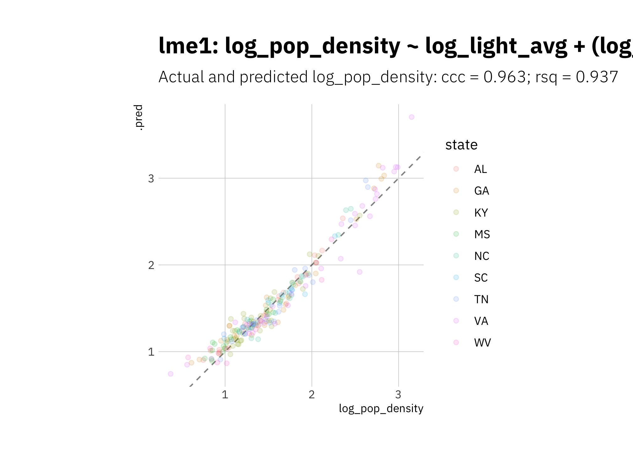
Figure 3.13: lme1 using holdout set
Again bs1 is performing quite well:
bs1_pred <- bs_wf_best %>%
  predict_on_holdout(., train_split, holdout)

bs1_metric_summary <- bind_rows(
  rsq(bs1_pred, truth = log_pop_density, estimate = .pred),
  ccc(bs1_pred, truth = log_pop_density, estimate = .pred)
) %>%
  mutate(model = unique(bs1_metric_summary$model))

bs1_pred %>%
  ggplot(aes(log_pop_density, .pred, color = state)) +
  geom_abline(lty = 2, alpha = 0.5) +
  geom_point(alpha = 0.15) +
  coord_fixed() +
  labs(title = glue("{bs1_metric_summary$model}"),
       subtitle = glue("Actual and predicted log_pop_density: ",
                       "{bs1_metric_summary[[2, 1]]} = {round(bs1_metric_summary[[2, 3]], 3)}",
                       "; {bs1_metric_summary[[1, 1]]} = {round(bs1_metric_summary[[1, 3]], 3)}")
  )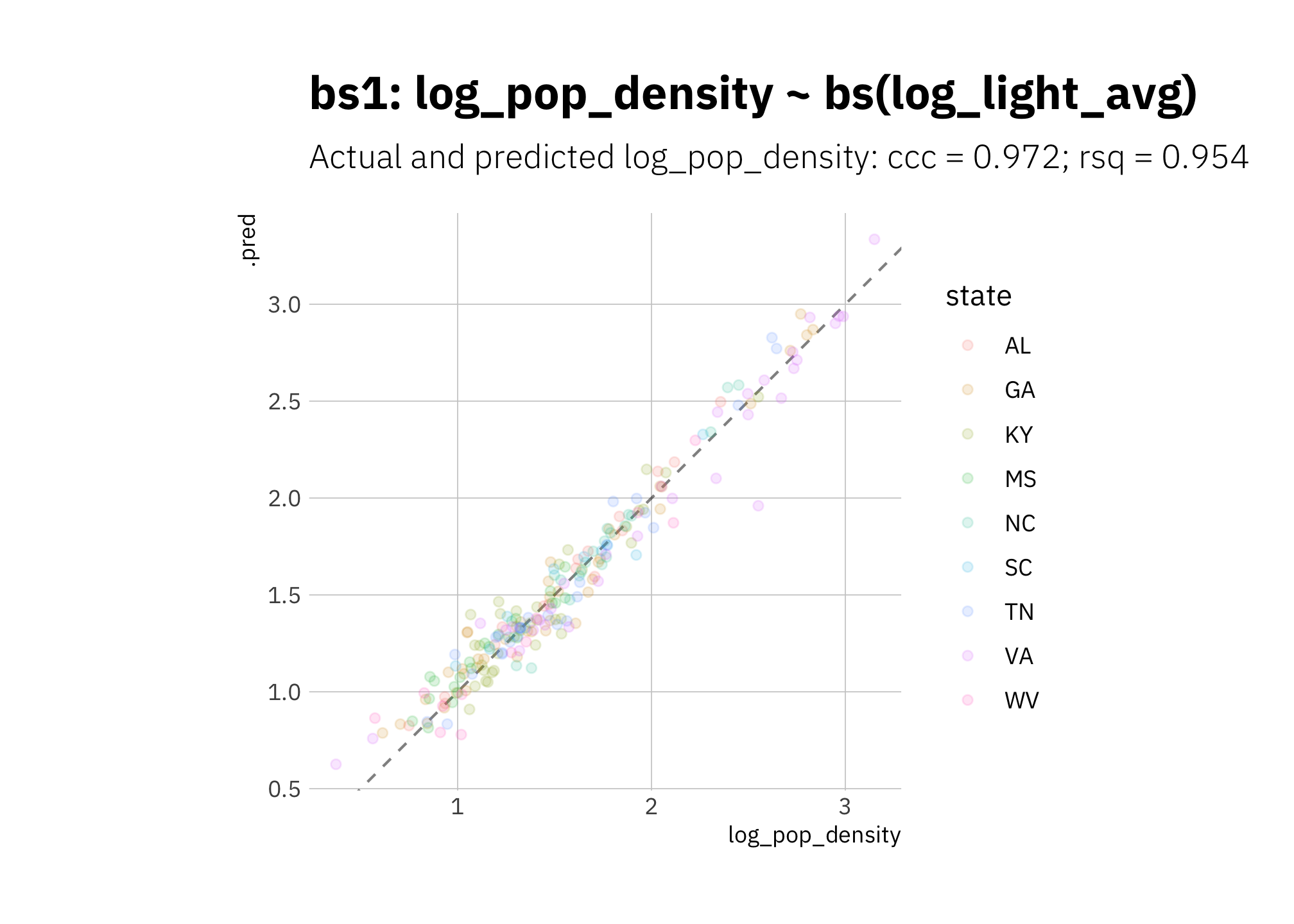
Figure 3.14: bs1 using holdout set
xg1 performance metrics are good, but the model is again systematically underestimating:
xg1_pred <- xg1_fit_best %>%
  predict_on_holdout(., train_split, holdout)

xg1_metric_summary <- bind_rows(
  rsq(xg1_pred, truth = log_pop_density, estimate = .pred),
  ccc(xg1_pred, truth = log_pop_density, estimate = .pred)
) %>%
  mutate(model = unique(xg1_metric_summary$model))

xg1_pred %>%
  ggplot(aes(log_pop_density, .pred, color = state)) +
  geom_abline(lty = 2, alpha = 0.5) +
  geom_point(alpha = 0.15) +
  coord_fixed() +
  labs(title = glue("{xg1_metric_summary$model}"),
       subtitle = glue("Actual and predicted log_pop_density: ",
                       "{xg1_metric_summary[[2, 1]]} = {round(xg1_metric_summary[[2, 3]], 3)}",
                       "; {xg1_metric_summary[[1, 1]]} = {round(xg1_metric_summary[[1, 3]], 3)}")
  )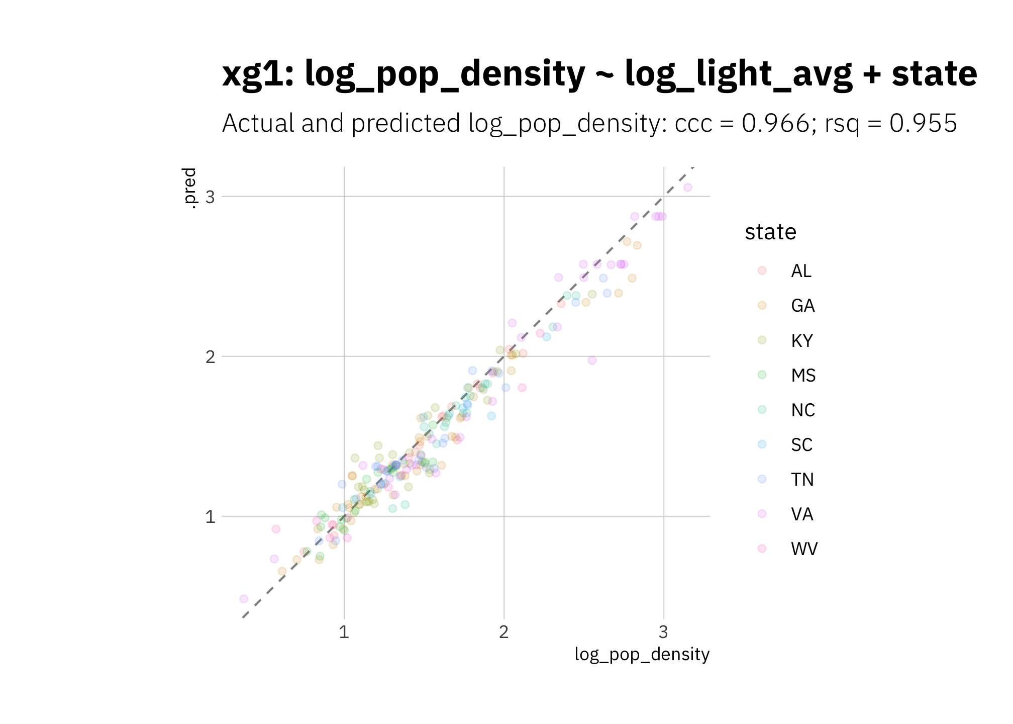
Figure 3.15: xg1 using holdout set
3.2.1 Summary: model evaluation using holdout data set
Results are similar for all models. The very simple lin3 is very competitive. I exclude lme1 from the next stage.
all_metrics <- bind_rows(
  lin3_metric_summary,
  pol1_metric_summary,
  lme1_metric_summary,
  bs1_metric_summary,
  xg1_metric_summary
)

model_levels = all_metrics %>%
  filter(.metric == "ccc") %>%
  arrange(.estimate) %>%
  pull(model)

all_metrics %>%
  mutate(model = factor(model, levels = model_levels)) %>%
  ggplot(aes(.estimate, model)) +
  geom_point() +
  geom_label(aes(label = str_pad(round(.estimate, 3),
                                 width = 5, side = "right", pad = "0")
                 ),
             size = 3, nudge_x = -0.1, hjust = 1) +
  expand_limits(x = 0) +
  facet_wrap(~ .metric, scales = "free_x") +
  theme(legend.position = "none",
        plot.title.position = "plot") +
  labs(title = "Model evaluation on holdout data set",
       x = "metric estimate",
       y = "")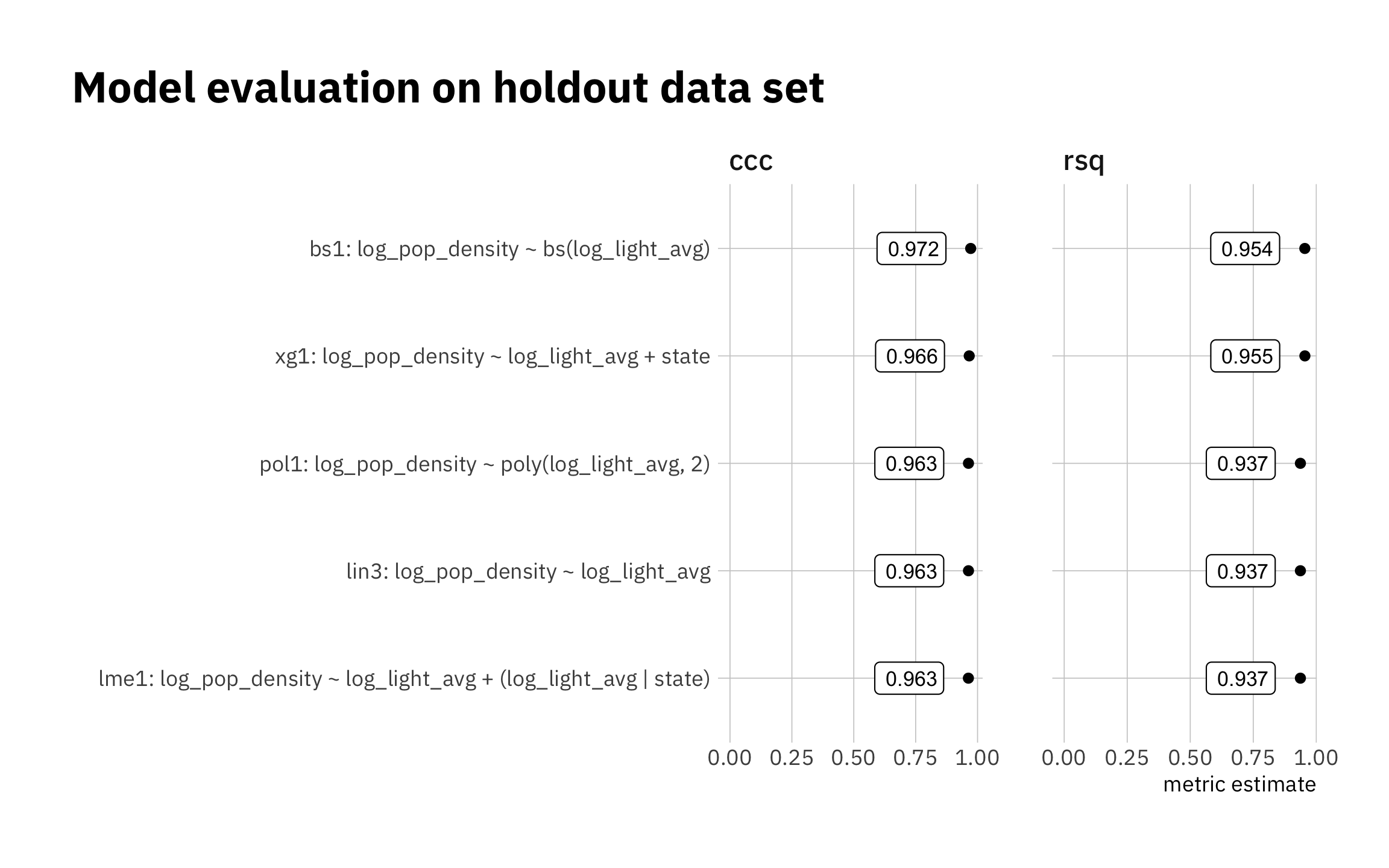
Figure 3.16: Summary of holdout results
all_metrics %>%
  dplyr::select(-.estimator) %>%
  arrange(.metric, desc(.estimate)) %>%
  gt() %>%
  tab_header(
  title = md("**Model evaluation on holdout data set**")
  ) %>%
  fmt_number(columns = .estimate,
decimals = 3)| Model evaluation on holdout data set | ||
|---|---|---|
| .metric | .estimate | model |
| ccc | 0.972 | bs1: log_pop_density ~ bs(log_light_avg) |
| ccc | 0.966 | xg1: log_pop_density ~ log_light_avg + state |
| ccc | 0.963 | lin3: log_pop_density ~ log_light_avg |
| ccc | 0.963 | pol1: log_pop_density ~ poly(log_light_avg, 2) |
| ccc | 0.963 | lme1: log_pop_density ~ log_light_avg + (log_light_avg | state) |
| rsq | 0.955 | xg1: log_pop_density ~ log_light_avg + state |
| rsq | 0.954 | bs1: log_pop_density ~ bs(log_light_avg) |
| rsq | 0.937 | lme1: log_pop_density ~ log_light_avg + (log_light_avg | state) |
| rsq | 0.937 | lin3: log_pop_density ~ log_light_avg |
| rsq | 0.937 | pol1: log_pop_density ~ poly(log_light_avg, 2) |
3.3 Comparing 2000 and 2010
I use the four remaining models to predict changes in log_pop_density in 2010 based on average county radiance log_light_avg in the same year, comparing performance on the holdout set with the 2010 assessment set.
lin3 looks pretty good, but the model overestimates high 2010 log_pop_density values.
lin3_pred <- lin3_wf %>%
  predict_on_holdout(., holdout, assess_df)

lin3_metric_summary <- bind_rows(
  rsq(lin3_pred, truth = log_pop_density, estimate = .pred),
  ccc(lin3_pred, truth = log_pop_density, estimate = .pred)
) %>%
  mutate(model = unique(lin3_metric_summary$model))

lin3_pred %>%
  ggplot(aes(log_pop_density, .pred, color = state)) +
  geom_abline(lty = 2, alpha = 0.5) +
  geom_point(alpha = 0.15) +
  coord_fixed() +
  labs(title = glue("{lin3_metric_summary$model}"),
       subtitle = glue("Actual and predicted log_pop_density: ",
                       "{lin3_metric_summary[[2, 1]]} = {round(lin3_metric_summary[[2, 3]], 3)}",
                       "; {lin3_metric_summary[[1, 1]]} = {round(lin3_metric_summary[[1, 3]], 3)}")
  )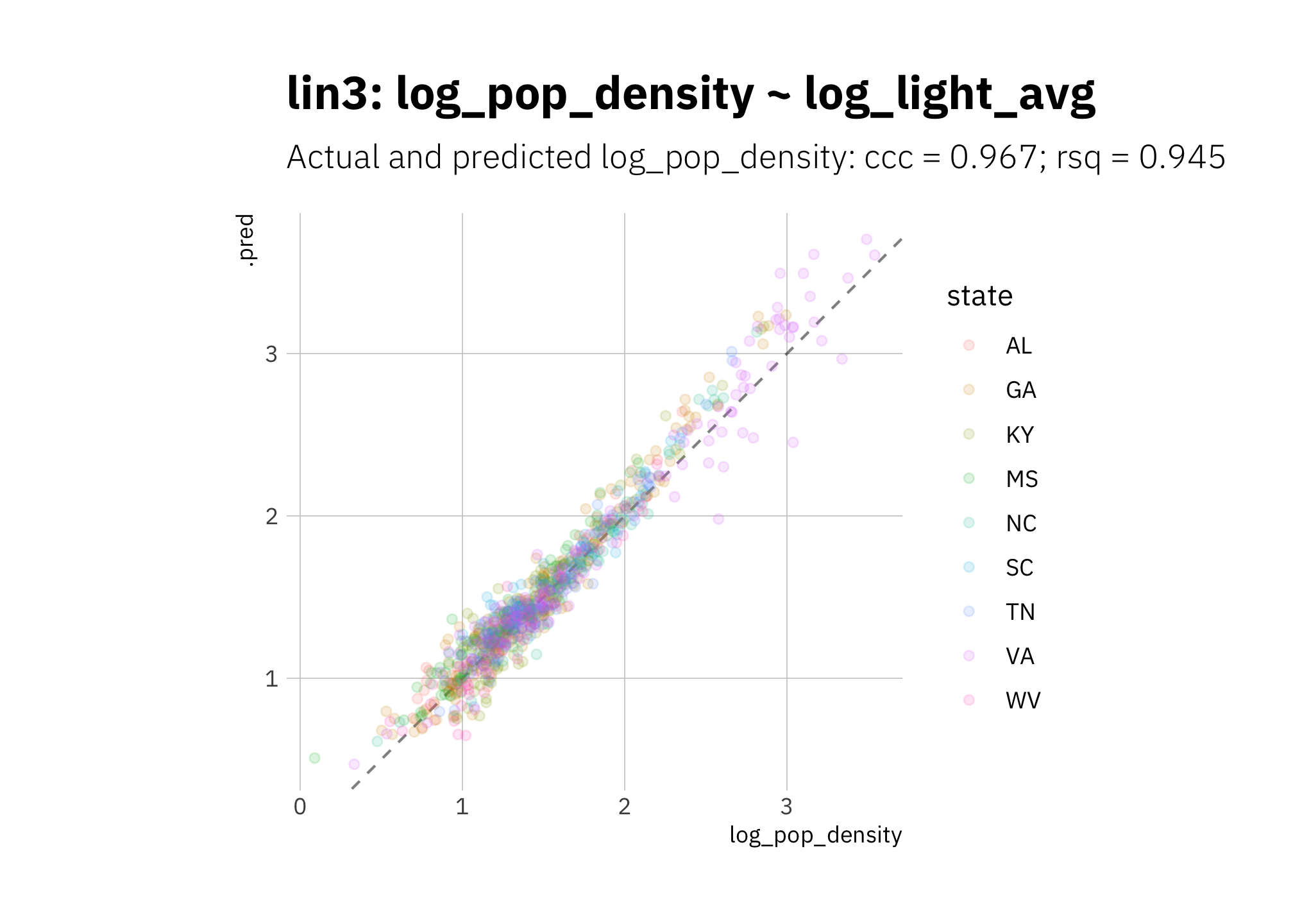
Figure 3.17: lin3 2010 assess set results
pol1 is underestimating low 2010 log_pop_density values and overestimating most other values:
pol1_pred <- pol1_wf %>%
  predict_on_holdout(., holdout, assess_df)

pol1_metric_summary <- bind_rows(
  rsq(pol1_pred, truth = log_pop_density, estimate = .pred),
  ccc(pol1_pred, truth = log_pop_density, estimate = .pred)
) %>%
  mutate(model = unique(pol1_metric_summary$model))

pol1_pred %>%
  ggplot(aes(log_pop_density, .pred, color = state)) +
  geom_abline(lty = 2, alpha = 0.5) +
  geom_point(alpha = 0.15) +
  coord_fixed() +
  labs(title = glue("{pol1_metric_summary$model}"),
       subtitle = glue("Actual and predicted log_pop_density: ",
                       "{pol1_metric_summary[[2, 1]]} = {round(pol1_metric_summary[[2, 3]], 3)}",
                       "; {pol1_metric_summary[[1, 1]]} = {round(pol1_metric_summary[[1, 3]], 3)}")
  )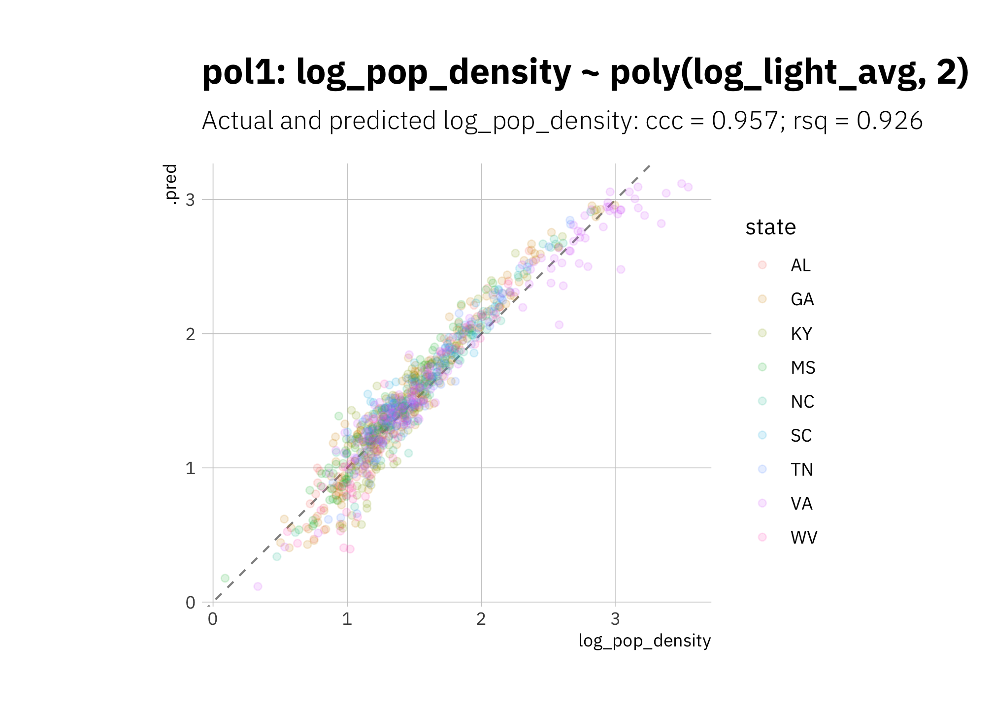
Figure 3.18: pol1 2010 assess set results
Like pol1, bs1 is underestimating low 2010 log_pop_density values and overestimating most other values:
bs1_pred <- bs_wf_best %>%
  predict_on_holdout(., holdout, assess_df)

bs1_metric_summary <- bind_rows(
  rsq(bs1_pred, truth = log_pop_density, estimate = .pred),
  ccc(bs1_pred, truth = log_pop_density, estimate = .pred)
) %>%
  mutate(model = unique(bs1_metric_summary$model))

bs1_pred %>%
  ggplot(aes(log_pop_density, .pred, color = state)) +
  geom_abline(lty = 2, alpha = 0.5) +
  geom_point(alpha = 0.15) +
  coord_fixed() +
  labs(title = glue("{bs1_metric_summary$model}"),
       subtitle = glue("Actual and predicted log_pop_density: ",
                       "{bs1_metric_summary[[2, 1]]} = {round(bs1_metric_summary[[2, 3]], 3)}",
                       "; {bs1_metric_summary[[1, 1]]} = {round(bs1_metric_summary[[1, 3]], 3)}")

  )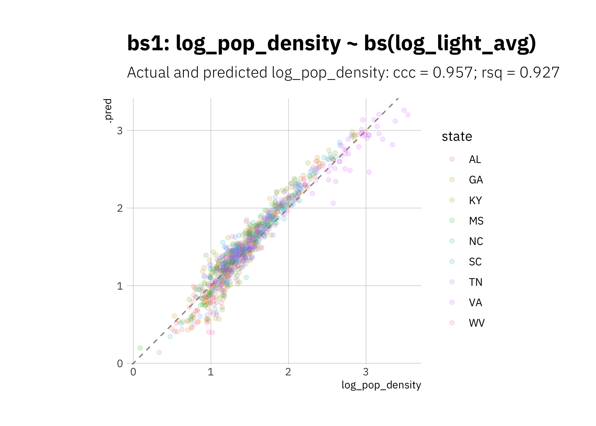
Figure 3.19: bs1 2010 assess set results
xg1 is underestimating low and high log_pop_density values:
xg1_pred <- xg1_fit_best %>%
  predict_on_holdout(., holdout, assess_df)

xg1_metric_summary <- bind_rows(
  rsq(xg1_pred, truth = log_pop_density, estimate = .pred),
  ccc(xg1_pred, truth = log_pop_density, estimate = .pred)
) %>%
  mutate(model = unique(xg1_metric_summary$model))

xg1_pred %>%
  ggplot(aes(log_pop_density, .pred, color = state)) +
  geom_abline(lty = 2, alpha = 0.5) +
  geom_point(alpha = 0.15) +
  coord_fixed() +
  labs(title = glue("{xg1_metric_summary$model}"),
       subtitle = glue("Actual and predicted log_pop_density: ",
                       "{xg1_metric_summary[[2, 1]]} = {round(xg1_metric_summary[[2, 3]], 3)}",
                       "; {xg1_metric_summary[[1, 1]]} = {round(xg1_metric_summary[[1, 3]], 3)}")
  )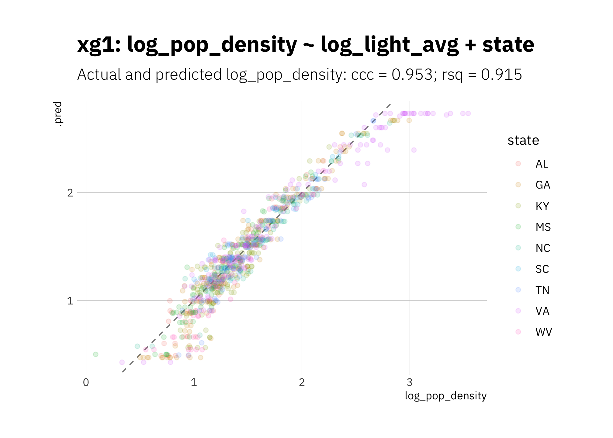
Figure 3.20: xg1 2010 assess set results
3.3.1 Summary: model performance on census 2010 data.
The simplest model lin3 perform slightly better, and our next-simplest odes. pol1, and bs1 are essentially equal. xg1 does worse at high and low log_pop_density values. This is a sign that xg1 may be overfitted on the training data. Even so, the difference in performance among the models are quite small.
Looking the absolute value of difference in means between predicted and true log_pop_density, I see all four models are performing similarly:
all_means <- bind_rows(
  with(lin3_pred, t.test(.pred, log_pop_density, paired = TRUE)) %>% tidy() %>%
    mutate(model = unique(lin3_metric_summary$model)),
  with(xg1_pred, t.test(.pred, log_pop_density, paired = TRUE)) %>% tidy() %>%
    mutate(model = unique(xg1_metric_summary$model)),
  with(pol1_pred, t.test(.pred, log_pop_density, paired = TRUE)) %>% tidy() %>%
    mutate(model = unique(pol1_metric_summary$model)),
  with(bs1_pred, t.test(.pred, log_pop_density, paired = TRUE)) %>% tidy() %>%
    mutate(model = unique(bs1_metric_summary$model))
) %>%
  rename(diff_in_means = estimate) %>%
  arrange(desc(abs(diff_in_means))) %>%
  mutate(model = as_factor(model)) # creates levels with current ordering

all_means %>%
  ggplot(aes(abs(diff_in_means), model)) +
  geom_errorbarh(aes(xmin = abs(conf.low), xmax = abs(conf.high), height = 0.1)) +
  geom_point() +
  theme(legend.position = "none",
        plot.title.position = "plot") +
  labs(title = "Difference in means between predicted and\nactual log_pop_density (2010 data)",
       subtitle = "T-test at 95% CI.",
       x = "difference in means",
       y = "")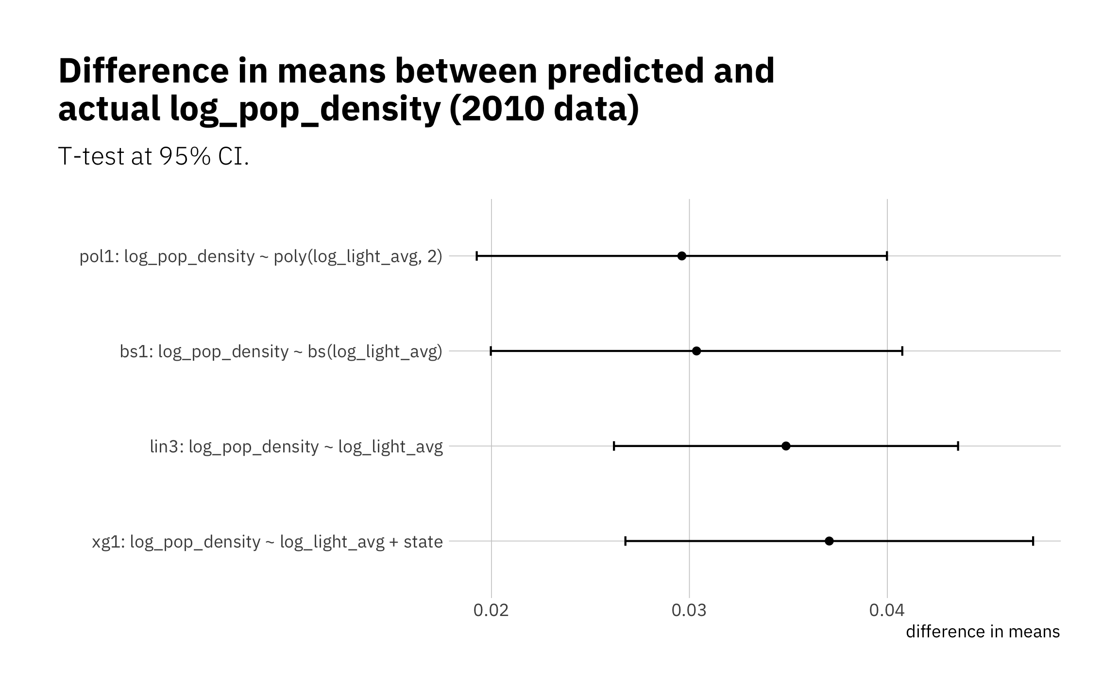
Figure 3.21: Differences in the means (predicted v actual)
all_metrics <- bind_rows(
  lin3_metric_summary,
  pol1_metric_summary,
  xg1_metric_summary,
  bs1_metric_summary
)

model_levels = all_metrics %>%
  filter(.metric == "ccc") %>%
  arrange(.estimate) %>%
  pull(model)

all_metrics %>%
  mutate(model = factor(model, levels = model_levels)) %>%
  ggplot(aes(.estimate, model)) +
  geom_point() +
  geom_label(aes(label = str_pad(round(.estimate, 3),
                                 width = 5, side = "right", pad = "0")
                 ),
             size = 3, nudge_x = -0.1, hjust = 1) +
  expand_limits(x = 0) +
  facet_wrap(~ .metric, scales = "free_x") +
  theme(legend.position = "none",
        plot.title.position = "plot") +
  labs(title = "Model evaluation on 2010 data",
       x = "metric estimate",
       y = "")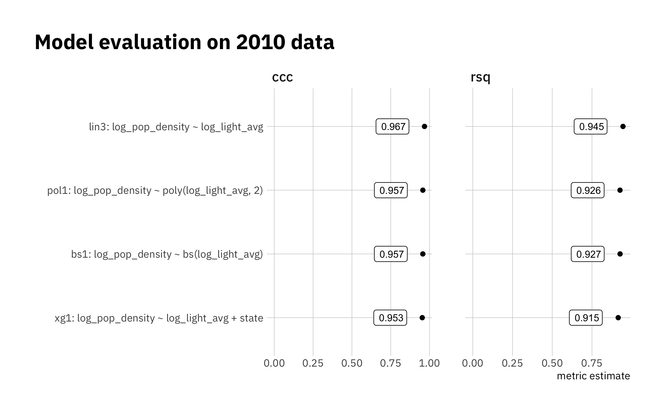
Figure 3.22: Holdout set results
all_metrics %>%
  dplyr::select(-.estimator) %>%
  arrange(.metric, desc(.estimate)) %>%
  gt() %>%
  tab_header(
  title = md("**Model evaluation on 2010 data**")
  ) %>%
  fmt_number(columns = c(.estimate),
decimals = 3)| Model evaluation on 2010 data | ||
|---|---|---|
| .metric | .estimate | model |
| ccc | 0.967 | lin3: log_pop_density ~ log_light_avg |
| ccc | 0.957 | pol1: log_pop_density ~ poly(log_light_avg, 2) |
| ccc | 0.957 | bs1: log_pop_density ~ bs(log_light_avg) |
| ccc | 0.953 | xg1: log_pop_density ~ log_light_avg + state |
| rsq | 0.945 | lin3: log_pop_density ~ log_light_avg |
| rsq | 0.927 | bs1: log_pop_density ~ bs(log_light_avg) |
| rsq | 0.926 | pol1: log_pop_density ~ poly(log_light_avg, 2) |
| rsq | 0.915 | xg1: log_pop_density ~ log_light_avg + state |
By Daniel Moul (heydanielmoul via gmail)
 This work is licensed under a Creative Commons Attribution 4.0 International License