Show the code
dta_nc <- dta |>
  filter(state == "NC")

dta_nc_2025 <- dta_nc |>
  filter(yr == 2025) |>
  reframe(n_stations = n(),
          n_chargers = sum(n_chargers),
          n_ev_network = n_distinct(ev_network)
)It can be helpful to zoom in on one place to see local dynamics. Below I look at North Carolina and then zoom in further to the Triangle area, where I live.
dta_nc <- dta |>
filter(state == "NC")
dta_nc_2025 <- dta_nc |>
filter(yr == 2025) |>
reframe(n_stations = n(),
n_chargers = sum(n_chargers),
n_ev_network = n_distinct(ev_network)
)At the end of 2025, there were 38 EV charging networks operating in North Carolina with 2054 stations and 6321 chargers1
ev_networks_nc <- dta_nc |>
  st_drop_geometry() |>
  filter(yr == 2025) |>
  reframe(n_chargers = sum(n_chargers),
          n_stations = n(),
          .by = ev_network) |>
  arrange(desc(n_chargers)) |>
  mutate(chargers_per_station = n_chargers / n_stations,
         rowid = row_number())

ev_networks_nc |>
  gt() |>
  tab_header(md("**EV Charging networks active in NC at end of 2025***")) |>
  fmt_number(columns = chargers_per_station,
decimals = 1)| EV Charging networks active in NC at end of 2025* | ||||
|---|---|---|---|---|
| ev_network | n_chargers | n_stations | chargers_per_station | rowid |
| ChargePoint Network | 1828 | 1002 | 1.8 | 1 |
| Non-Networked | 1092 | 332 | 3.3 | 2 |
| Tesla | 1054 | 88 | 12.0 | 3 |
| Blink Network | 605 | 164 | 3.7 | 4 |
| EV Connect | 395 | 132 | 3.0 | 5 |
| Tesla Destination | 189 | 71 | 2.7 | 6 |
| LOOP | 134 | 32 | 4.2 | 7 |
| AMPUP | 131 | 20 | 6.5 | 8 |
| Electrify America | 121 | 21 | 5.8 | 9 |
| eVgo Network | 75 | 21 | 3.6 | 10 |
| ENVIROSPARK | 67 | 16 | 4.2 | 11 |
| IONNA | 64 | 7 | 9.1 | 12 |
| CHARGEUP | 63 | 17 | 3.7 | 13 |
| FORD_CHARGE | 58 | 17 | 3.4 | 14 |
| SWTCH | 56 | 13 | 4.3 | 15 |
| NOODOE | 55 | 5 | 11.0 | 16 |
| CIRCLE_K | 54 | 12 | 4.5 | 17 |
| RED_E | 51 | 9 | 5.7 | 18 |
| RIVIAN_ADVENTURE | 36 | 6 | 6.0 | 19 |
| EVGATEWAY | 33 | 8 | 4.1 | 20 |
| CHARGELAB | 32 | 8 | 4.0 | 21 |
| SHELL_RECHARGE | 24 | 10 | 2.4 | 22 |
| UNIVERSAL | 18 | 9 | 2.0 | 23 |
| ZEFNET | 15 | 3 | 5.0 | 24 |
| MERCEDES_BENZ | 10 | 6 | 1.7 | 25 |
| STAY_N_CHARGE | 10 | 5 | 2.0 | 26 |
| AUTEL | 8 | 1 | 8.0 | 27 |
| AMPED_UP | 6 | 1 | 6.0 | 28 |
| FLO | 6 | 3 | 2.0 | 29 |
| RIVIAN_WAYPOINTS | 6 | 3 | 2.0 | 30 |
| OpConnect | 4 | 2 | 2.0 | 31 |
| VIALYNK | 4 | 2 | 2.0 | 32 |
| TURNONGREEN | 4 | 2 | 2.0 | 33 |
| EVMATCH | 3 | 2 | 1.5 | 34 |
| IN_CHARGE | 3 | 1 | 3.0 | 35 |
| EVOKE | 3 | 1 | 3.0 | 36 |
| EPIC_CHARGING | 2 | 1 | 2.0 | 37 |
| CHAEVI | 2 | 1 | 2.0 | 38 |
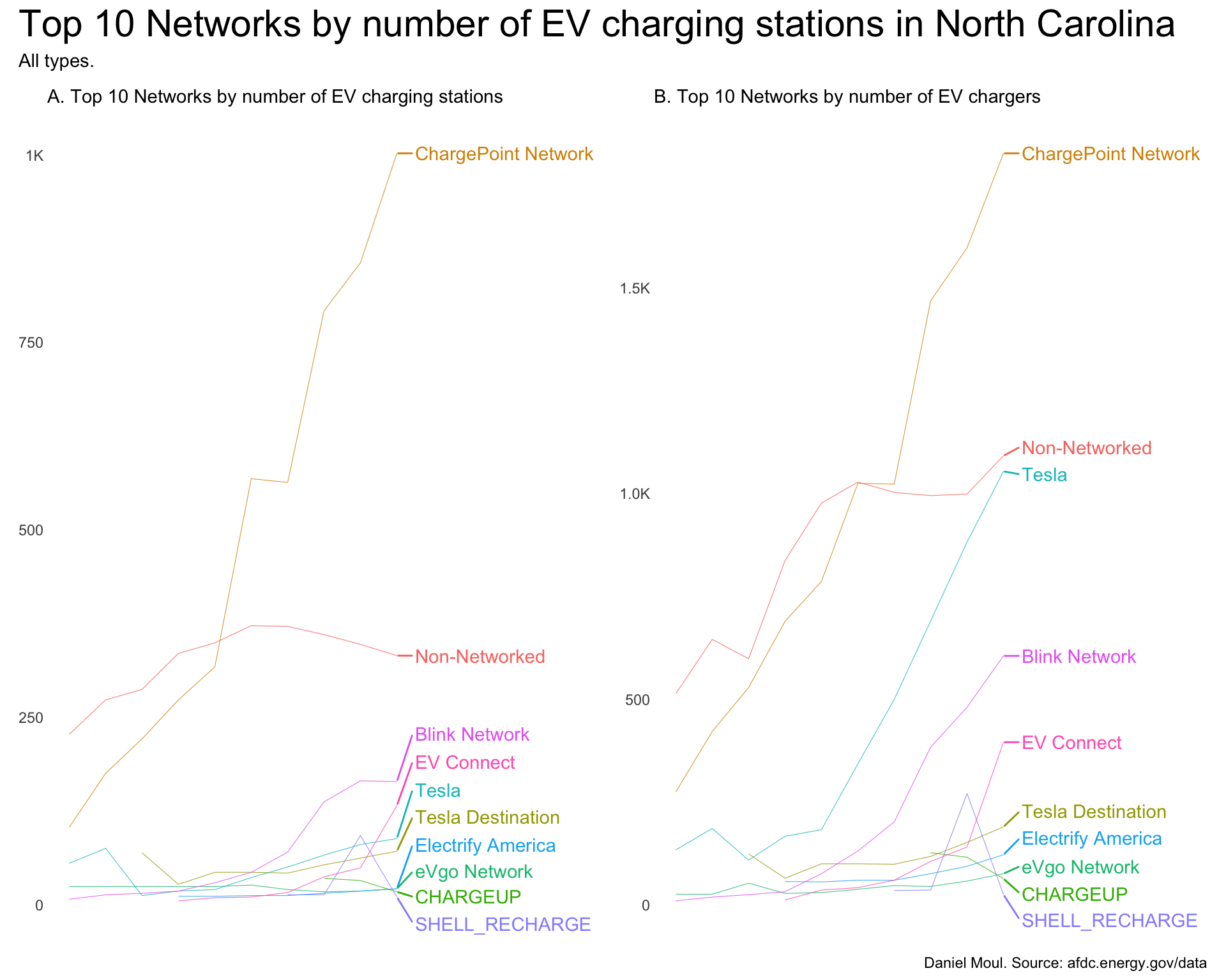
There were three networks (plus “Non-Networked”) with more than 500 chargers at end of 2025 (Figure 4.1 panel B).
ev_network_top_10_stations_nc <- dta_nc |>
  count(ev_network, sort = TRUE) |>
  head(10)

ev_network_top_10_chargers_nc <- dta_nc |>
  count(ev_network, wt = n_chargers, sort = TRUE) |>
  head(10)

dta_for_plot <- dta_nc |>
  filter(ev_network %in% ev_network_top_10_stations_nc$ev_network) |>
  reframe(
    n_stations = n(),
    n_chargers = sum(n_chargers),
    chargers_per_station = n_chargers / n_stations,
    .by = c(yr, state, ev_network)
  ) |>
  mutate(ev_network = fct_reorder(ev_network, -n_stations, max))

dta_labels_for_plot <- dta_for_plot |>
  filter(yr == 2025)

p1 <- dta_for_plot |>
  ggplot() +
  geom_line(
    aes(yr, n_stations, group = ev_network, color = ev_network),
    linewidth = 0.2,
    alpha = 0.8) +
  geom_text_repel(
    data = dta_labels_for_plot,
    aes(x = yr,
        y = n_stations,
        label = ev_network,
        color = ev_network),
    nudge_x = 0.5,
    direction = "y",
    hjust = 0) +
  scale_x_discrete(labels = year_labels) +
  scale_y_continuous(labels = label_number(scale_cut = cut_short_scale())) +
  guides(color = "none") +
  coord_cartesian(xlim = c(NA, 2030)) +
  labs(
    subtitle = "A. Top 10 Networks by number of EV charging stations ",
    x = NULL,
    y = NULL
  )

dta_for_plot2 <- dta_nc |>
  filter(ev_network %in% ev_network_top_10_chargers_nc$ev_network) |>
  reframe(
    n_stations = n(),
    n_chargers = sum(n_chargers),
    chargers_per_station = n_chargers / n_stations,
    .by = c(yr, state, ev_network)
  ) |>
  mutate(ev_network = fct_reorder(ev_network, -n_stations, max))

dta_labels_for_plot2 <- dta_for_plot2 |>
  filter(yr == 2025)

p2 <- dta_for_plot2 |>
  ggplot() +
  geom_line(
    aes(yr, n_chargers, group = ev_network, color = ev_network),
    linewidth = 0.2,
    alpha = 0.8) +
  geom_text_repel(
    data = dta_labels_for_plot2,
    aes(x = yr,
        y = n_chargers,
        label = ev_network,
        color = ev_network),
    nudge_x = 0.5,
    direction = "y",
    hjust = 0) +
  scale_x_discrete(labels = year_labels) +
  scale_y_continuous(labels = label_number(scale_cut = cut_short_scale())) +
  guides(color = "none") +
  coord_cartesian(xlim = c(NA, 2030)) +
  labs(
    subtitle = "B. Top 10 Networks by number of EV chargers",
    x = NULL,
    y = NULL
  )

p1 + p2 +
  plot_annotation(
    title = "Top 10 Networks by number of EV charging stations in North Carolina",
    subtitle = "All types.",
    caption = my_caption
  )
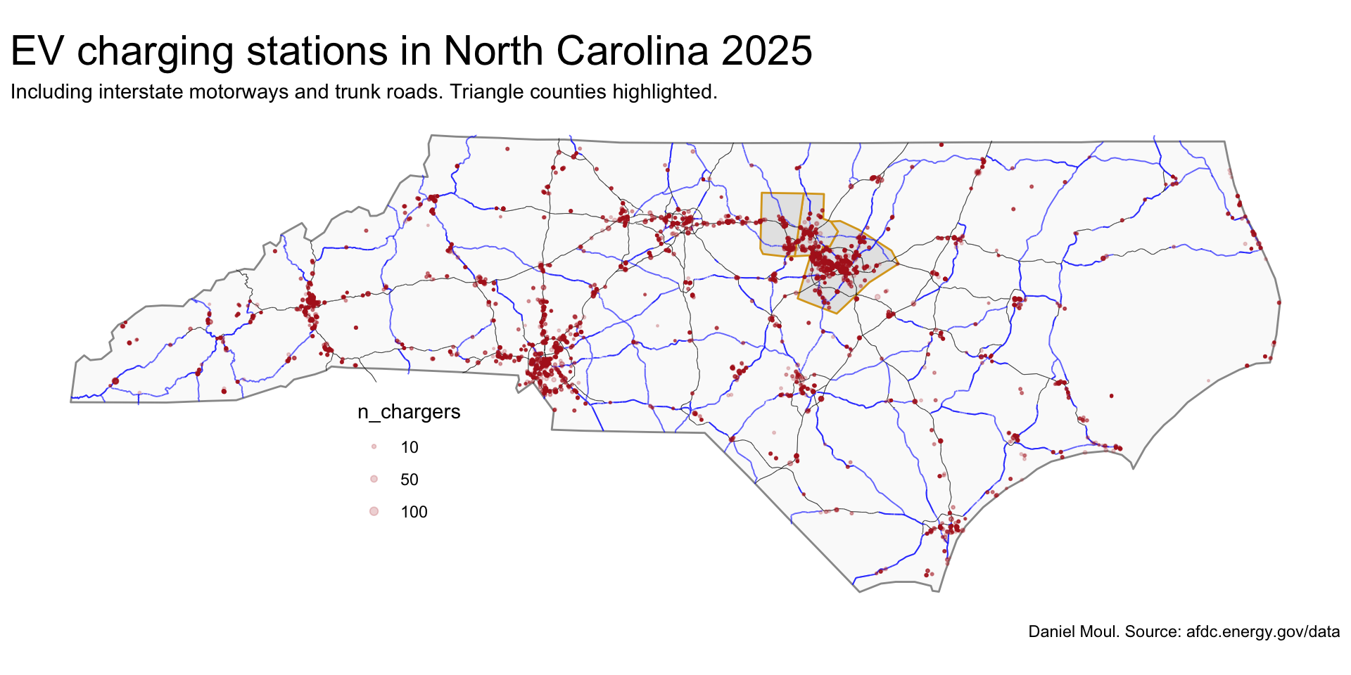
Chargers are where the people are (as you would expect) plus on common travel routes (Figure 4.2). The counties making up the core of the Triangle are highlighted.
nc_border <- state_boundaries_sf |>
  filter(state_abb == "NC")

dta_nc_sf <- dta_nc |>
  st_as_sf(coords = c("longitude", "latitude"),
           crs = "WGS84") |>
  st_transform(crs = my_proj) %>%
  # need to get rid of some bad points
  st_crop(st_bbox(nc_border)) # much faster
  # st_intersection(nc_border, .) # this works but is very slow

nc_counties <- us_counties(states = "NC") |>
  select(-state_name) |>
  st_transform(crs = my_proj)

nc_triangle <- nc_counties |>
  filter(name %in% c("Orange",
                     "Wake",
                     "Durham"))

nc_triangle_bbox <- st_bbox(nc_triangle)

dta_triangle_sf <- dta_nc_sf |>
  st_crop(nc_triangle_bbox)

dta_triangle_no_geom <- dta_triangle_sf |>
  st_drop_geometry()

ev_networks_triangle <- dta_triangle_no_geom |>
  st_drop_geometry() |>
  filter(yr == 2025) |>
  reframe(n_chargers = sum(n_chargers),
          n_stations = n(),
          .by = ev_network) |>
  arrange(desc(n_chargers)) |>
  mutate(chargers_per_station = n_chargers / n_stations,
         rowid = row_number())

facility_type_2025 <- dta_triangle_no_geom |>
  filter(yr == 2025) |>
  reframe(
    n_stations = n(),
    n_chargers = sum(n_chargers),
    .by = facility_type
  ) |>
  replace_na(list(facility_type = "Unspecified"))

facility_type_ev_network_2025 <- dta_triangle_no_geom |>
  filter(yr == 2025) |>
  reframe(
    n_stations = n(),
    n_chargers = sum(n_chargers),
    .by = c(ev_network, facility_type)
  ) |>
  replace_na(list(facility_type = "Unspecified"))


get_pop_2020_tract_tmp <-  function(proj) {
  get_decennial(
    geography = c("tract"),
    variables = c(pop = "P001001"),
    state = "NC",
    county = c("Orange", "Durham", "Wake"),
    # year = 2020,
    geometry = TRUE,
    # output = "wide"
  ) #|>
    clean_names() |>
    separate(name, into = c("tract_name", "county", "state"), sep = ", ") |>
    mutate(tract_name = str_extract(tract_name, "\\d+(\\.\\d+)?"),
           county = str_extract(county, "^.+(?= County)")
    ) |>
    select(-c(state)) |>
    mutate(year = 2000) |>
    st_transform(crs = proj)
}

v2020_dhc <- load_variables(2020, "dhc")

census_tract_triangle_2020 <- get_decennial(
    geography = c("tract"),
    variables = c("P1_001N"),
    state = "NC",
    county = c("Orange", "Durham", "Wake"),
    year = 2020,
    geometry = TRUE,
    cb = FALSE,
    cache_table = TRUE
  ) |>
  rename(pop = value) |>
  clean_names() |>
  mutate(county = str_extract(name, "Orange|Durham|Wake"),
         area_m2 = as.numeric(st_area(geometry)),
         area_mi2 = 3.861E-07 * area_m2,
         density_mi2 = pop / area_mi2)

####### OSM data: NC state roads
fname <- here("data/processed/nc-highways.rds")

if(!file.exists(fname)) {

  nc_highways_motorways <- st_bbox(nc_border) |>
    opq()%>%
    add_osm_feature(key = "highway",
                    value = c("motorway", "trunk")) %>%
    osmdata_sf()

  write_rds(nc_highways_motorways$osm_lines |>
      st_simplify(dTolerance = 100),
      fname)

} else {

  nc_highways_motorways <- read_rds(fname)

}

# Is it faster to covert to spatVector, use mask(), and convert back to sf instead of st_intersection()? YES

# nc_highways_motorways_lines <- nc_highways_motorways$osm_lines |>
#   select(osm_id, highway, ref, geometry) |>
#   st_transform(crs = my_proj) |>
#   st_crop(nc_border) %>%
#   # TODO: do I need to do st_intersection() here? YES
#   st_intersection(nc_border, .) |> # this works but is very slow
#   mutate(highway = factor(highway, levels = c("motorway", "trunk"),
#                           ordered = TRUE))

nc_highways_motorways_lines <- nc_highways_motorways |>
  select(osm_id, highway, ref, geometry) |>
  st_transform(crs = my_proj) |>
  filter(!st_is_empty(geometry)) |>
  vect() |>
  crop(nc_border) %>%
  mask(vect(nc_border)) |>
  st_as_sf() |>
  mutate(highway = factor(highway, levels = c("motorway", "trunk"),
                          ordered = TRUE))

####### OSM data: Triangle roads
fname <- here("data/processed/triangle-highways.rds")

if(!file.exists(fname)) {

  triangle_highways_motorways <- nc_triangle_bbox |>
    opq()%>%
    add_osm_feature(key = "highway",
                    value = c("motorway", "trunk", "primary")) %>%
    osmdata_sf()

  write_rds(triangle_highways_motorways$osm_lines  |>
      st_simplify(dTolerance = 100),
      fname)

} else {

  triangle_highways_motorways <- read_rds(fname)

}

triangle_highways_motorways_lines <- triangle_highways_motorways |>
  select(osm_id, highway, ref, geometry) |>
  st_transform(crs = my_proj) |>
  st_crop(nc_triangle_bbox) |>
  mutate(highway = factor(highway, levels = c("primary", "trunk", "motorway"),
ordered = TRUE))ggplot() +
geom_sf(
data = nc_border,
linewidth = 0.5,
color = "grey60",
fill = "grey98") +
geom_sf(
data = nc_triangle,
linewidth = 0.5,
# lty = 2,
color = "goldenrod" #"grey40"
) +
geom_sf(
data = nc_highways_motorways_lines,
aes(linewidth = highway,
color = highway),
alpha = 0.6) +
geom_sf(
data = dta_nc_sf,
aes(size = n_chargers),
color = "firebrick",
alpha = 0.2) +
scale_linewidth_discrete(range = c(0.15, 0.35)) +
scale_color_manual(values = c("black", "blue")) + # "darkslateblue")) +
scale_size_continuous(breaks = c(10, 50, 100),
range = c(0.25, 2.0)) +
guides(size = guide_legend(position = "inside"),
linewidth = "none",
color = "none") +
theme(legend.position.inside = c(0.3, 0.3),
axis.text = element_blank()) +
labs(
title = "EV charging stations in North Carolina 2025",
subtitle = "Including interstate motorways and trunk roads. Triangle counties highlighted.",
caption = my_caption
)
There were 23 EV charging networks active in the Triangle area at the end of 2025. Among them they offer 626 stations and 1880 chargers.
ev_networks_triangle |>
  gt() |>
  tab_header(md("**EV Charging networks active in NC Triangle in 2025***")) |>
  fmt_number(columns = chargers_per_station,
decimals = 1)| EV Charging networks active in NC Triangle in 2025* | ||||
|---|---|---|---|---|
| ev_network | n_chargers | n_stations | chargers_per_station | rowid |
| ChargePoint Network | 713 | 373 | 1.9 | 1 |
| Non-Networked | 290 | 72 | 4.0 | 2 |
| Blink Network | 233 | 55 | 4.2 | 3 |
| Tesla | 149 | 11 | 13.5 | 4 |
| EV Connect | 96 | 29 | 3.3 | 5 |
| LOOP | 70 | 17 | 4.1 | 6 |
| SWTCH | 47 | 9 | 5.2 | 7 |
| NOODOE | 41 | 2 | 20.5 | 8 |
| Electrify America | 37 | 6 | 6.2 | 9 |
| IONNA | 36 | 5 | 7.2 | 10 |
| eVgo Network | 35 | 11 | 3.2 | 11 |
| Tesla Destination | 34 | 7 | 4.9 | 12 |
| SHELL_RECHARGE | 18 | 7 | 2.6 | 13 |
| CHARGEUP | 16 | 4 | 4.0 | 14 |
| FORD_CHARGE | 16 | 4 | 4.0 | 15 |
| AMPUP | 15 | 6 | 2.5 | 16 |
| AUTEL | 8 | 1 | 8.0 | 17 |
| ZEFNET | 8 | 1 | 8.0 | 18 |
| AMPED_UP | 6 | 1 | 6.0 | 19 |
| UNIVERSAL | 4 | 2 | 2.0 | 20 |
| CHARGELAB | 4 | 1 | 4.0 | 21 |
| EVGATEWAY | 2 | 1 | 2.0 | 22 |
| RED_E | 2 | 1 | 2.0 | 23 |
Are the chargers located in the US Census tracts with the greatest density? Only partly (Figure 4.3):
ggplot() +
  geom_sf(
    data = census_tract_triangle_2020,
    aes(fill = density_mi2),
    color = NA,
    ) +
  geom_sf(
    data = nc_triangle,
    # fill = "grey98",
    fill = NA,
    lty = 2,
    linewidth = 0.3,
    color = "grey70") +
  geom_sf(
    data = triangle_highways_motorways_lines,
    aes(linewidth = highway,
        color = highway),
    alpha = 0.6) +
  geom_sf(
    data = dta_triangle_sf,
    aes(size = n_chargers),
    color = "firebrick",
    alpha = 0.2) +
  scale_size_continuous(breaks = c(1, 10, 20),
                        range = c(0.25, 2.0)) +
  scale_linewidth_discrete(range = c(0.15, 0.5)) +
  scale_color_manual(values = c("grey", "black", "blue")) +  #"darkslateblue")) +
  scale_fill_gradient(low ="white",
                      high = "dodgerblue") +
  guides(size = guide_legend(position = "right"),
         fill = "none") +
  theme(axis.text = element_blank()) +
  labs(
    title = "EV charging stations in the NC Triangle in 2025",
    subtitle = "Orange, Durham, and Wake counties with major roads (motorways, trunk, primary)\nand population density of US Census tracts",
    caption = paste0(my_caption, ", US Census 2020")
  )
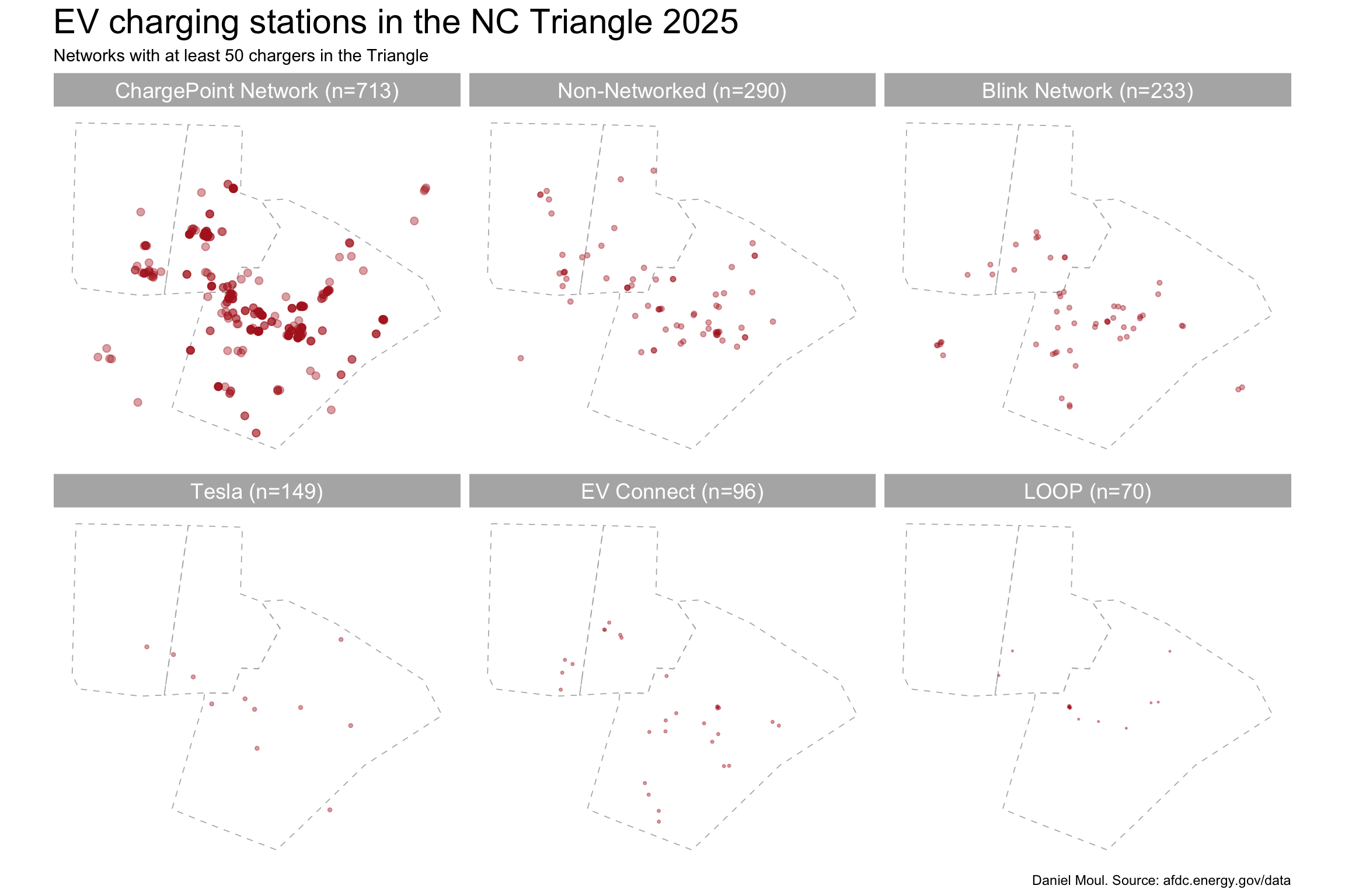
dta_for_plot_sf <- dta_triangle_sf |>
  left_join(ev_networks_nc |>
              rename(n_chargers_ev_network = n_chargers),
            by = "ev_network") |>
  filter(yr == 2025) |>
  mutate(n_stations = n(),
         n_chargers_sum = sum(n_chargers),
         ev_network_facet = glue("{ev_network} (n={n_chargers_sum})"),
         .by = ev_network) |>
  filter(n_chargers_sum > 50) |>
  mutate(ev_network_facet = fct_reorder(ev_network_facet, -n_chargers_sum))

ggplot() +
  geom_sf(
    data = nc_triangle,
    fill = NA,
    lty = 2,
    linewidth = 0.3,
    color = "grey70") +
  geom_sf(
    data = dta_for_plot_sf,
    aes(size = n_chargers_sum),
    color = "firebrick",
    alpha = 0.4) +
  scale_size_continuous(breaks = c(1, 10, 20),
                        range = c(0.25, 2.0)) +
  guides(size = guide_legend(position = "top")) +
  facet_wrap( ~ ev_network_facet) +
  theme(axis.text = element_blank()) +
  labs(
    title = "EV charging stations in the NC Triangle 2025",
    subtitle = "Networks with at least 50 chargers in the Triangle",
    caption = my_caption
  )
dta_for_plot <- dta_triangle_sf |>
  st_drop_geometry() |>
  reframe(
    n_stations = n(),
    n_chargers = sum(n_chargers),
    chargers_per_station = n_chargers / n_stations,
    .by = c(yr, state, ev_network)
  ) |>
  group_by(yr) |>
  mutate(n_networks = n()) |>
  arrange(n_chargers) |>
  mutate(ordering = row_number()) |>
  ungroup()

max_x = max(dta_for_plot$n_chargers)

dta_for_plot |>
  ggplot(aes(n_chargers, ordering)) +
  geom_point(
    size = 1.5,
    color = "firebrick",
    alpha = 0.6) +
  geom_text(aes(label = ev_network),
            hjust = 0,
            nudge_x = 40) +
  guides(color = "none") +
  coord_cartesian(xlim = c(NA, max_x + 1000)) +
  facet_wrap(~ yr, nrow = 2) +
  labs(
    title = glue("EV charging networks active in the Triangle each year 2016-2025",
                 "\nby number of chargers"),
    subtitle = "Ordered by number of chargers",
    x = "Numberof chargers",
    y = NULL
  )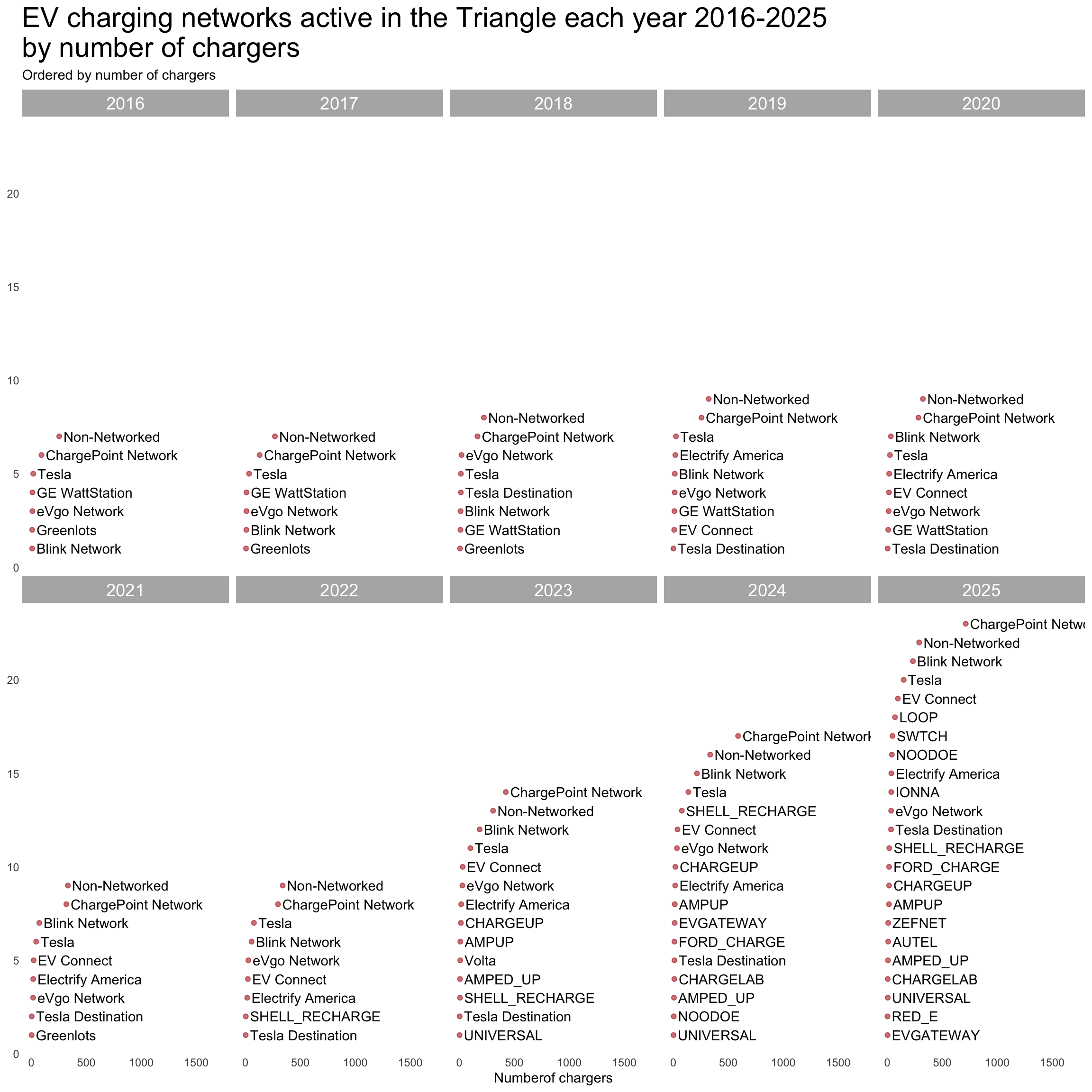
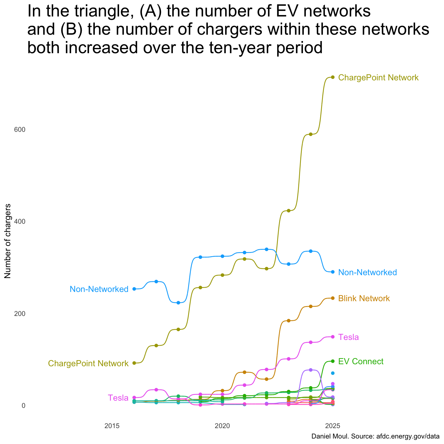
Focusing on the EV charging networks with the most chargers (Figure 4.6):
dta_labels_for_plot <- dta_for_plot |>
  filter(yr == min(yr)) |>
  arrange(desc(n_chargers)) |>
  head(3)

dta_labels_for_plot_right <- dta_for_plot |>
  filter(yr == max(yr)) |>
  arrange(desc(n_chargers)) |>
  head(5)

dta_for_plot |>
  ggplot() +
  geom_text(
    data = dta_labels_for_plot,
    aes(x = yr,
        y = n_chargers,
        label = ev_network,
        color = ev_network),
    # direction = "y",
    nudge_x = -0.25,
    hjust = 1) +
  geom_text(
    data = dta_labels_for_plot_right,
    aes(x = yr,
        y = n_chargers,
        label = ev_network,
        color = ev_network),
    # direction = "y",
    nudge_x = 0.25,
    hjust = 0) +
  geom_point(
    aes(x = yr,
        y = n_chargers,
        color = ev_network
    )) +
  geom_bump(
    aes(x = yr,
        y = n_chargers,
        color = ev_network
    )) +
  guides(color = "none") +
  coord_cartesian(xlim = c(2012, 2029)) +
  labs(
    title = glue("In the triangle, (A) the number of EV networks",
                 "\nand (B) the number of chargers within these networks",
                 "\nboth increased over the ten-year period"),
    x = NULL,
    y = "Number of chargers",
    caption = my_caption
  )
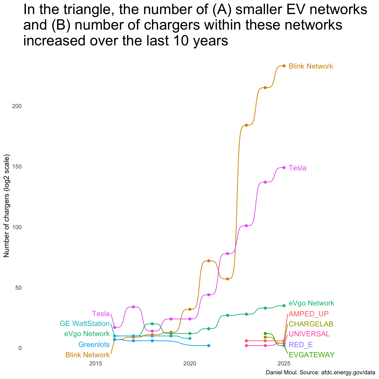
Looking at the smallest networks in 2016 and 2025 (Figure 4.7):
dta_labels_for_plot_left <- dta_for_plot |>
  filter(yr == min(yr)) |>
  slice_min(order_by = n_chargers,
            n = 5)

dta_labels_for_plot_right <- dta_for_plot |>
  filter(yr == max(yr)) |>
  slice_min(order_by = n_chargers,
            n = 5)

dta_labels_for_plot <- dta_for_plot |>
  filter(ev_network %in% union(dta_labels_for_plot_left$ev_network, dta_labels_for_plot_right$ev_network)) |>
  select(yr, ev_network, n_chargers) |>
  filter(yr == min(yr) | yr == max(yr))

dta_for_plot |>
  filter(ev_network %in% union(dta_labels_for_plot$ev_network, dta_labels_for_plot_right$ev_network)) |>
  ggplot() +
  geom_text_repel(
    data = dta_labels_for_plot,
    aes(x = if_else(yr == min(yr),
                    yr,
                    NA),
        y = n_chargers,
        label = ev_network,
        color = ev_network),
    direction = "y",
    nudge_x = -0.25,
    hjust = 1,
    na.rm = TRUE) +
  geom_text_repel(
    data = dta_labels_for_plot,
    aes(x = if_else(yr == max(yr),
                    yr,
                    NA),
        y = n_chargers,
        label = ev_network,
        color = ev_network),
    direction = "y",
    nudge_x = 0.25,
    hjust = 0,
    na.rm = TRUE) +
  geom_point(
    aes(x = yr,
        y = n_chargers,
        color = ev_network
    )) +
  geom_bump(
    aes(x = yr,
        y = n_chargers,
        color = ev_network
    )) +
  guides(color = "none") +
  coord_cartesian(xlim = c(2012, 2029)) +
  labs(
    title = glue("In the triangle, the number of (A) smaller EV networks",
                 "\nand (B) number of chargers within these networks",
                 "\nincreased over the last 10 years"),
    x = NULL,
    y = "Number of chargers (log2 scale)",
    caption = my_caption
  )
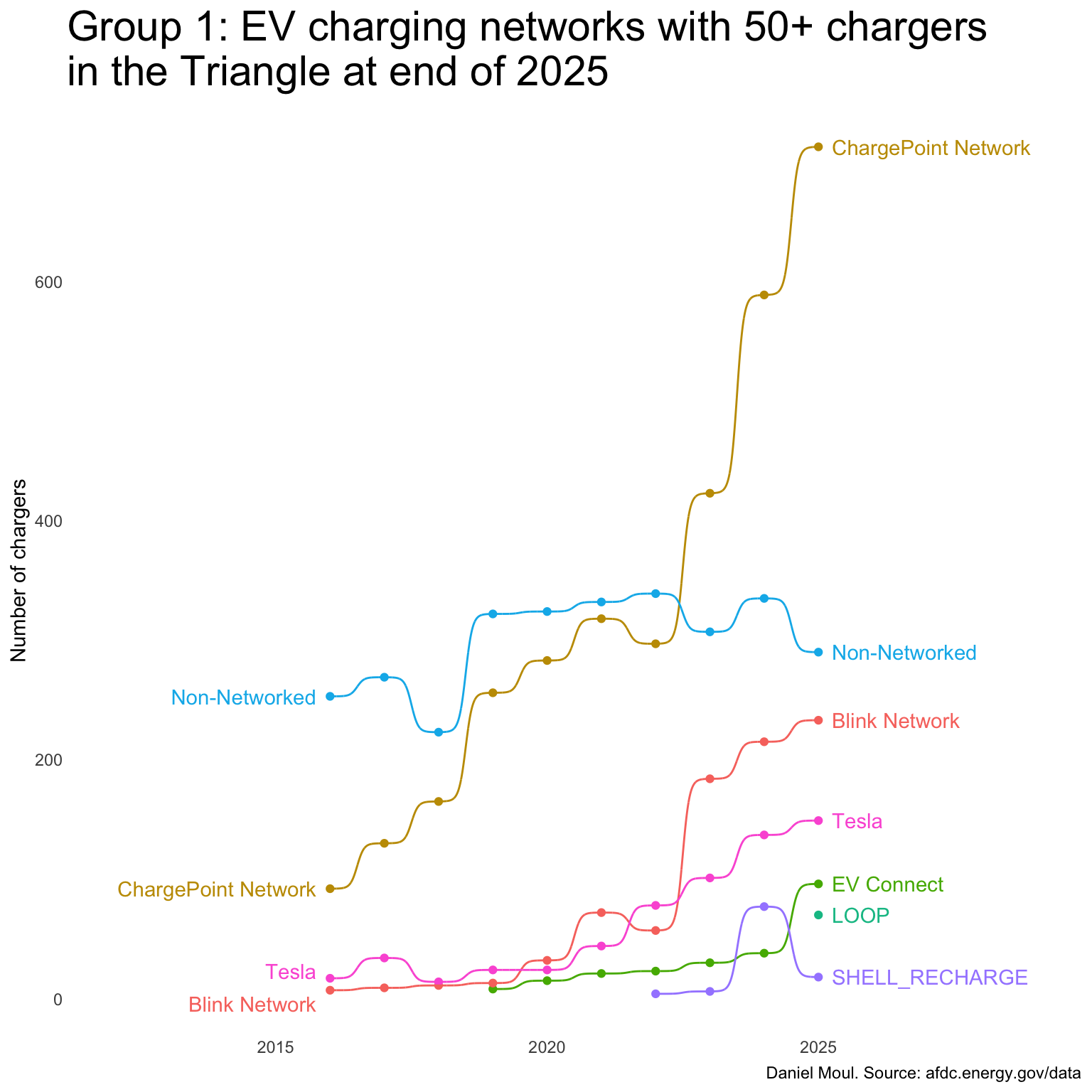
Three bump charts are based on number of chargers in the Triangle at end of 2025:
dta_labels_for_plot <- dta_for_plot |>
  filter(any(n_chargers >= 50),
         .by = ev_network)

dta_for_plot |>
  filter(ev_network %in% dta_labels_for_plot$ev_network) |>
  ggplot() +
  geom_text_repel(
    data = dta_labels_for_plot,
    aes(x = if_else(yr == min(yr),
                    yr,
                    NA),
        y = n_chargers,
        label = ev_network,
        color = ev_network),
    direction = "y",
    nudge_x = -0.25,
    hjust = 1,
    na.rm = TRUE) +
  geom_text_repel(
    data = dta_labels_for_plot,
    aes(x = if_else(yr == max(yr),
                    yr,
                    NA),
        y = n_chargers,
        label = ev_network,
        color = ev_network),
    direction = "y",
    nudge_x = 0.25,
    hjust = 0,
    na.rm = TRUE) +
  geom_point(
    aes(x = yr,
        y = n_chargers,
        color = ev_network
    )) +
  geom_bump(
    aes(x = yr,
        y = n_chargers,
        color = ev_network
    )) +
  guides(color = "none") +
  coord_cartesian(xlim = c(2012, 2029)) +
  labs(
    title = glue("Group 1: EV charging networks with 50+ chargers",
                 "\nin the Triangle at end of 2025"),
    x = NULL,
    y = "Number of chargers",
    caption = my_caption
  )
dta_labels_for_plot <- dta_for_plot |>
  filter(!any(n_chargers >= 50),
         .by = ev_network) |>
  filter(any(between(n_chargers, 10, 49)),
         .by = ev_network) |>
  filter(yr == min(yr) | yr == max(yr))

dta_for_plot |>
  filter(ev_network %in% dta_labels_for_plot$ev_network) |>
  ggplot() +
  geom_text_repel(
    data = dta_labels_for_plot,
    aes(x = if_else(yr == min(yr),
                    yr,
                    NA),
        y = n_chargers,
        label = ev_network,
        color = ev_network),
    direction = "y",
    nudge_x = -0.25,
    hjust = 1,
    na.rm = TRUE) +
  geom_text_repel(
    data = dta_labels_for_plot,
    aes(x = if_else(yr == max(yr),
                    yr,
                    NA),
        y = n_chargers,
        label = ev_network,
        color = ev_network),
    direction = "y",
    nudge_x = 0.25,
    hjust = 0,
    na.rm = TRUE) +
  geom_point(
    aes(x = yr,
        y = n_chargers,
        color = ev_network
    )) +
  geom_bump(
    aes(x = yr,
        y = n_chargers,
        color = ev_network
    )) +
  guides(color = "none") +
  coord_cartesian(xlim = c(2012, 2029)) +
  labs(
    title = glue("Group 2: EV charging networks with 10-49 chargers",
                 "\nin the Triangle at end of 2025"),
    x = NULL,
    y = "Number of chargers",
    caption = my_caption
  )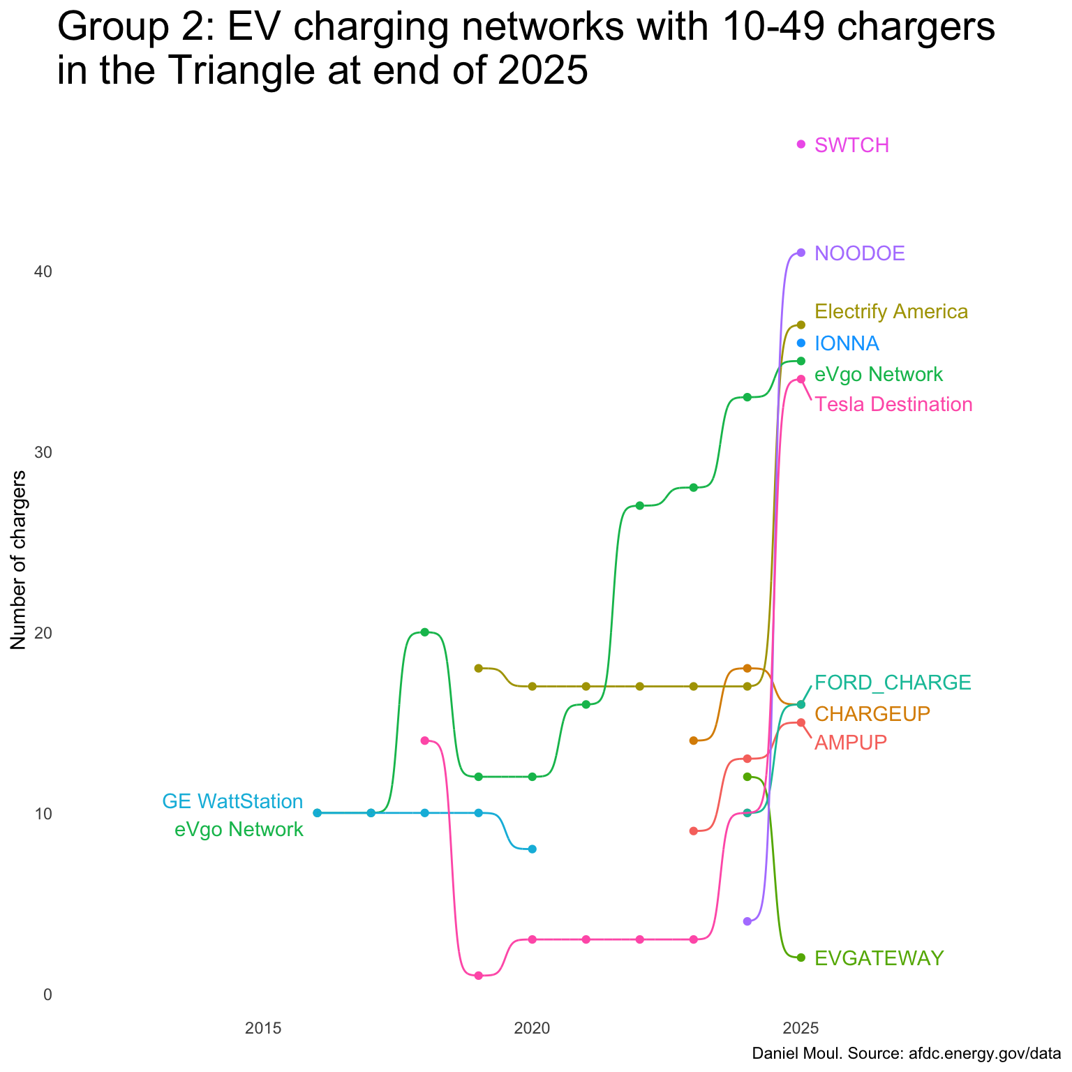
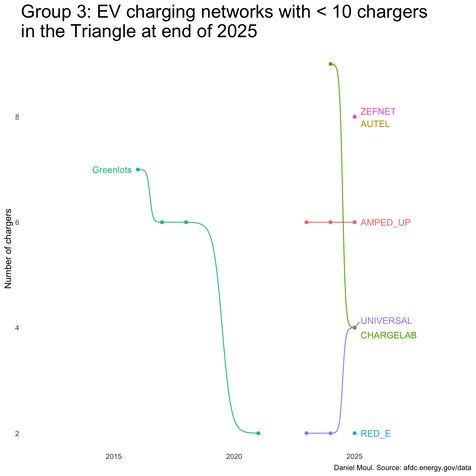
dta_labels_for_plot <- dta_for_plot |>
  filter(!any(n_chargers >= 10),
         .by = ev_network) |>
  filter(yr == min(yr) | yr == max(yr))

dta_for_plot |>
  filter(ev_network %in% dta_labels_for_plot$ev_network) |>
  ggplot() +
  geom_text_repel(
    data = dta_labels_for_plot,
    aes(x = if_else(yr == min(yr),
                    yr,
                    NA),
        y = n_chargers,
        label = ev_network,
        color = ev_network),
    direction = "y",
    nudge_x = -0.25,
    hjust = 1,
    na.rm = TRUE) +
  geom_text_repel(
    data = dta_labels_for_plot,
    aes(x = if_else(yr == max(yr),
                    yr,
                    NA),
        y = n_chargers,
        label = ev_network,
        color = ev_network),
    direction = "y",
    nudge_x = 0.25,
    hjust = 0,
    na.rm = TRUE) +
  geom_point(
    aes(x = yr,
        y = n_chargers,
        color = ev_network
    )) +
  geom_bump(
    aes(x = yr,
        y = n_chargers,
        color = ev_network
    )) +
  guides(color = "none") +
  coord_cartesian(xlim = c(2012, 2029)) +
  labs(
    title = glue("Group 3: EV charging networks with < 10 chargers",
                 "\nin the Triangle at end of 2025"),
    x = NULL,
    y = "Number of chargers",
    caption = my_caption
  )
n_unspecified_stations <- facility_type_2025$n_stations[facility_type_2025$facility_type == "Unspecified"]
n_unspecified_chargers <- facility_type_2025$n_chargers[facility_type_2025$facility_type == "Unspecified"]

pct_unspecified_stations <- n_unspecified_stations / sum(facility_type_2025$n_stations)
pct_unspecified_chargers <- n_unspecified_chargers / sum(facility_type_2025$n_chargers)
Unfortunately most facility_type values are unspecified: 81% of the stations and 71% chargers. And LOOP shows facility_type = “OTHER” for all their stations in NC (but not nationally). Nonetheless, it’s interesting to see what facility_type values are in the data set (Table 4.3):
facility_type_2025 |>
  arrange(desc(n_chargers)) |>
  gt() |>
  tab_options(table.font.size = 11) |>
tab_header(md("**Facility locations for EV charging stations in the Triangle**"))| Facility locations for EV charging stations in the Triangle | ||
|---|---|---|
| facility_type | n_stations | n_chargers |
| Unspecified | 506 | 1331 |
| OFFICE_BLDG | 12 | 99 |
| SHOPPING_CENTER | 9 | 78 |
| OTHER | 17 | 70 |
| MOTOR_POOL, FLEET GARAGE | 7 | 42 |
| PARKING_LOT | 6 | 39 |
| HOTEL, INN, B&B | 13 | 35 |
| MUNI_GOV | 9 | 35 |
| CAR_DEALER | 9 | 20 |
| PARKING_GARAGE | 4 | 17 |
| PUBLIC | 4 | 16 |
| GAS_STATION | 2 | 14 |
| GROCERY | 2 | 14 |
| FED_GOV | 7 | 12 |
| RESTAURANT | 2 | 10 |
| MULTI_UNIT_DWELLING | 1 | 10 |
| HOSPITAL | 2 | 8 |
| MUSEUM | 2 | 8 |
| COLLEGE_CAMPUS | 2 | 5 |
| STREET_PARKING | 3 | 4 |
| PARK | 2 | 4 |
| LIBRARY | 2 | 4 |
| REC_SPORTS_FACILITY | 2 | 3 |
| WORKPLACE | 1 | 2 |
Some EV Networks report more facility_type data than others. Some seems to avoid reporting this information altogether–perhaps for competitive reasons.
##| column: page-right

facility_type_ev_network_2025 |>
  mutate(reporting = if_else(facility_type == "Unspecified",
                             "unspecified",
                             "reported")
  ) |>
  reframe(
    n_stations = sum(n_stations),
    n_chargers = sum(n_chargers),
    .by = c(ev_network, reporting)
  ) |>
  pivot_wider(
    names_from = reporting,
    values_from = c(n_stations, n_chargers),
    values_fill = 0) |>
  mutate(
    pct_stations_unspecified = n_stations_unspecified / (n_stations_reported + n_stations_unspecified),
    pct_chargers_unspecified = n_chargers_unspecified / (n_chargers_reported + n_chargers_unspecified)
  ) |>
  relocate(c(pct_stations_unspecified, pct_chargers_unspecified),
           .before = n_stations_reported) |>
  arrange(desc(pct_stations_unspecified), desc(n_chargers_unspecified)) %>%
  set_names(., nm = str_replace_all(names(.), "_", " ")) |>
  gt() |>
  tab_options(table.font.size = 11) |>
  tab_header(md("**Availability of `facility_type` data for EV charging stations in the Triangle**")) |>
  fmt_percent(columns = starts_with("pct"),
              decimals = 0)
Availability of facility_type data for EV charging stations in the Triangle |
||||||
|---|---|---|---|---|---|---|
| ev network | pct stations unspecified | pct chargers unspecified | n stations reported | n stations unspecified | n chargers reported | n chargers unspecified |
| ChargePoint Network | 100% | 100% | 0 | 373 | 0 | 713 |
| Blink Network | 100% | 100% | 0 | 55 | 0 | 233 |
| EV Connect | 100% | 100% | 0 | 29 | 0 | 96 |
| NOODOE | 100% | 100% | 0 | 2 | 0 | 41 |
| Electrify America | 100% | 100% | 0 | 6 | 0 | 37 |
| IONNA | 100% | 100% | 0 | 5 | 0 | 36 |
| eVgo Network | 100% | 100% | 0 | 11 | 0 | 35 |
| SHELL_RECHARGE | 100% | 100% | 0 | 7 | 0 | 18 |
| CHARGEUP | 100% | 100% | 0 | 4 | 0 | 16 |
| ZEFNET | 100% | 100% | 0 | 1 | 0 | 8 |
| CHARGELAB | 100% | 100% | 0 | 1 | 0 | 4 |
| EVGATEWAY | 100% | 100% | 0 | 1 | 0 | 2 |
| Tesla Destination | 71% | 91% | 2 | 5 | 3 | 31 |
| Tesla | 18% | 24% | 9 | 2 | 113 | 36 |
| Non-Networked | 6% | 9% | 68 | 4 | 265 | 25 |
| AMPUP | 0% | 0% | 6 | 0 | 15 | 0 |
| AMPED_UP | 0% | 0% | 1 | 0 | 6 | 0 |
| UNIVERSAL | 0% | 0% | 2 | 0 | 4 | 0 |
| SWTCH | 0% | 0% | 9 | 0 | 47 | 0 |
| FORD_CHARGE | 0% | 0% | 4 | 0 | 16 | 0 |
| AUTEL | 0% | 0% | 1 | 0 | 8 | 0 |
| LOOP | 0% | 0% | 17 | 0 | 70 | 0 |
| RED_E | 0% | 0% | 1 | 0 | 2 | 0 |
I am considering “Non-Networked one of the networks.↩︎