3  Modeling failure rate

Show the code

data_for_model <- dta_working_set |>
  mutate(median_km_driven_10K = median_km_driven / 10000) |>
  filter(any(model_year >= 2015),
         .by = brand) |>
  filter(n_model_years_brand >= 3) |>
  mutate(brand = fct_reorder(brand, failure_rate, mean))

3.1 Unfair average failure rates

Because failure_rate is influenced by distance driven and vehicle age (see Section A.1.2 Causal graph), a simple list of average failure rates by brand (Table 3.1) can be misleading. For example:

1. Brands with relatively more vehicles in older models years will have “unfairly” higher failure rates.

2. The lowest quality vehicles may be withdrawn from service relatively earlier than higher quality cars, “unfairly” reducing the lowest quality brands’ failure rates.

3. If brands mostly offer expensive sports cars that are driven less than average, then these brands will have “unfairly” low failure rates.

Show the code

##| column: page-right

data_for_model |>
  summarize(avg_failure_rate = weighted.mean(failure_rate, w = inspection_count),
            model_years_in_data = paste0(min(model_year), "-", max(model_year)),
            .by = brand) |>
  arrange(avg_failure_rate) |>
  mutate(rank = rank(avg_failure_rate)) |>
  gt() |>
  tab_header(md("**Brands ranked by average failure rate over all model years**")) |>
  fmt_number(columns = avg_failure_rate,
             decimals = 2)

Table 3.1: Brands ranked by average failure rate (not a fair ranking)

Brands ranked by average failure rate over all model years
brand	avg_failure_rate	model_years_in_data	rank
Porsche	0.09	2007-2018	1
Lexus	0.11	2007-2017	2
Suzuki	0.13	2007-2018	3
Toyota	0.13	2007-2018	4
Audi	0.14	2007-2018	5
Mini	0.15	2007-2018	6
Seat	0.16	2007-2018	7
Skoda	0.16	2007-2018	8
Honda	0.16	2007-2018	9
Tesla Motors	0.16	2015-2017	10
Mitsubishi	0.17	2007-2018	11
Volvo	0.17	2007-2018	12
VW	0.19	2007-2018	13
Opel	0.20	2007-2018	14
Subaru	0.21	2007-2018	15
Hyundai	0.21	2007-2018	16
Ford	0.21	2007-2018	17
BMW	0.22	2007-2018	18
MB	0.22	2007-2018	19
Kia	0.23	2007-2018	20
Jaguar Land Rover	0.23	2007-2017	21
Mazda	0.24	2007-2018	22
Nissan	0.27	2007-2018	23
Peugeot	0.28	2007-2018	24
Dacia	0.29	2010-2018	25
Renault	0.29	2007-2018	26
Citroen	0.30	2007-2018	27
Alfa Romeo	0.30	2007-2017	28
Fiat	0.31	2007-2017	29

3.2 Linear regressions

If we accept that inspection failure rate is a good proxy for brand quality, it’s possible to identify relative brand quality by accounting for these factors using regression analysis.

3.2.1 The two simplest models

Show the code

mod1 <- data_for_model |>
  lm(failure_rate ~ vehicle_age,
     data = _)

mod2 <- data_for_model |>
  lm(failure_rate ~ median_km_driven_10K,
     data = _)

According to Table 3.2

• For every one year increase in vehicle_age, the failure_rate went up by 2.5%.

• For every 10K km driven (median_km_driven_10K), the failure_rate increased by 1%.

Show the code

p1 <- bind_cols(
  tidy(mod1,
       conf.int = my_ci) |>
  select(term, estimate, std.error, p.value, conf.low, conf.high),
  glance(mod1) |>
  select(adj.r.squared, sigma, logLik, AIC, BIC, nobs)
) |> mutate(model = "mod1",
            formula = "lm(failure_rate ~ vehicle_age)")

p2 <- bind_cols(
  tidy(mod2,
       conf.int = my_ci) |>
  select(term, estimate, std.error, p.value, conf.low, conf.high),
  glance(mod2) |>
  select(adj.r.squared, sigma, logLik, AIC, BIC, nobs)
) |> mutate(model = "mod2",
            formula = "lm(failure_rate ~ median_km_driven_10K)")

bind_rows(p1, p2) |>
  relocate(c(model, formula), .before = term) |>
  filter(term != "(Intercept)") |>
  gt() |>
  tab_options(table.font.size = 10) |>
  fmt_number(columns = c(estimate, std.error, p.value, conf.low, conf.high, adj.r.squared, sigma),
             decimals = 3) |>
  fmt_number(columns = c( logLik, AIC, BIC),
             decimals = 0)

Table 3.2: Simple linear models compared

model	formula	term	estimate	std.error	p.value	conf.low	conf.high	adj.r.squared	sigma	logLik	AIC	BIC	nobs
mod1	lm(failure_rate ~ vehicle_age)	vehicle_age	0.025	0.001	0.000	0.024	0.026	0.557	0.079	1,730	−3,453	−3,437	1539
mod2	lm(failure_rate ~ median_km_driven_10K)	median_km_driven_10K	0.010	0.000	0.000	0.009	0.011	0.368	0.094	1,456	−2,907	−2,891	1539

Show the code

  # relatively higher R^2 and logLik indicates better fit
  # relatively lower AIC indicates better fit
  # relatively lower BIC indicates better fit

Regressing with vehicle_age provides a better fit than median_km_driven_10K

• Relatively higher \(R^2\) and log likelihood
• Relatively lower AIC and BIC

This is because vehicle_age encompasses failures due to age as well as a lot of the information about distance driven. See Section A.1.2 Causal graph and Table 1.3 High correlation among vehicle_age, median_km_driven and average_km_driven.

3.2.2 Relative brand quality in Finland

Show the code

my_lm_vehicle_age <- function(x) {
  lm(failure_rate ~ vehicle_age,
           data = x)
}

mod1_set <- data_for_model %>%
  filter(n_model_years_brand >= brands_cutoff_modeling_min) |>
  nest(data = c(failure_rate, vehicle_age),
       .by = brand) |>
  mutate(mod1 = map(data, my_lm_vehicle_age),
         tidyinfo = map(mod1, tidy,
                        conf.int = TRUE,
                        conf.level = my_ci)
         )

mod1_set_summary <- mod1_set |>
  select(brand, tidyinfo) |>
  unnest(tidyinfo) |>
  select(-statistic)

my_lm_km_driven <- function(x) {
  lm(failure_rate ~ median_km_driven_10K,
           data = x)
}

mod2_set <- data_for_model %>%
  filter(n_model_years_brand >= brands_cutoff_modeling_min) |>
  nest(data = c(failure_rate, median_km_driven_10K),
       .by = brand) |>
  mutate(mod1 = map(data, my_lm_km_driven),
         tidyinfo = map(mod1, tidy,
                        conf.int = TRUE,
                        conf.level = my_ci)
         )

mod2_set_summary <- mod2_set |>
  select(brand, tidyinfo) |>
  unnest(tidyinfo) |>
  select(-statistic)

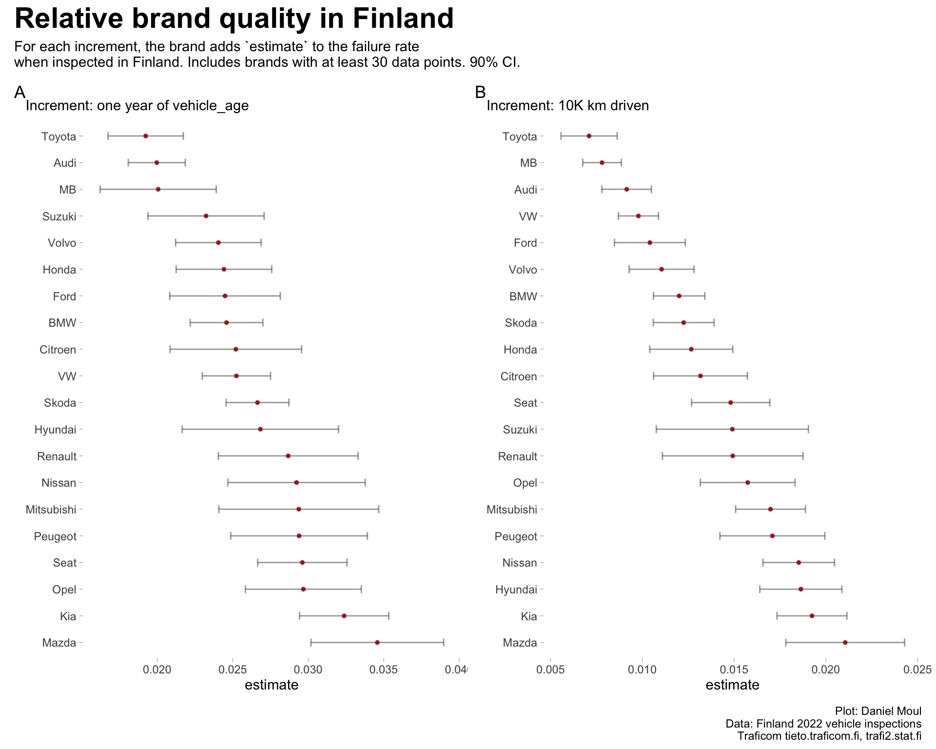
For each brand separately, I calculated lm(failure_rate ~ vehicle_age) and lm(failure_rate ~ median_km_driven_10K) and present them in Figure 3.1. I excluded brands that did not have at least 30 data points.

Given the wide range of the 90% confidence intervals, a relative difference in brand quality can be determined in the regression with vehicle_age only for the highest and lowest quality brands (where the intervals do not overlap in panel A). The narrower confidence intervals in the regression using median_km_driven_10K (panel B) provide a larger useful set of relative higher-quality and lower-quality brands.

Show the code

p1 <- mod1_set_summary |>
  filter(term != "(Intercept)") |>
  mutate(term = fct_reorder(brand, -estimate)) |>
  ggplot() +
  geom_errorbarh(aes(xmin = conf.low, xmax = conf.high, y = term),
                 height = 0.3,
                 linewidth = 0.5, alpha = 0.4,
                 show.legend = FALSE) +
  geom_point(aes(x = estimate, y = term),
             size = 1, color = "firebrick",
             show.legend = FALSE) +
  labs(
    subtitle = "Increment: one year of vehicle_age",
    y = NULL,
    tag = "A"
  )

p2 <- mod2_set_summary |>
  filter(term != "(Intercept)") |>
  mutate(term = fct_reorder(brand, -estimate)) |>
  ggplot() +
  geom_errorbarh(aes(xmin = conf.low, xmax = conf.high, y = term),
                 height = 0.3,
                 linewidth = 0.5, alpha = 0.4,
                 show.legend = FALSE) +
  geom_point(aes(x = estimate, y = term),
             size = 1, color = "firebrick",
             show.legend = FALSE) +
  labs(
    subtitle = "Increment: 10K km driven",
    y = NULL,
    tag = "B"
  )

p1 + p2 + 
  plot_annotation(
    title = "Relative brand quality in Finland",
    subtitle = glue("For each increment, the brand adds `estimate` to the failure rate",
                    "\nwhen inspected in Finland. Includes brands with at least {brands_cutoff_modeling_min} data points.",
                    " {percent(my_ci)} CI."),
    caption = my_caption
  )

Figure 3.1: Relative brand quality determined using linear regression

The tables below include the estimates and confidence intervals plotted in in Figure 3.1.

Show the code

mod1_set_summary |>
  filter(term != "(Intercept)") |>
  mutate(plus_minus = (conf.high - conf.low) / 2) |>
  select(-term) |>
  gt() |>
  fmt_number(columns = c(estimate:plus_minus),
             decimals = 3) |>
  tab_source_note(md(glue("*For each brand, calculated separately: lm(failure_rate ~ vehicle_age)* at {my_ci} CI")))
mod2_set_summary |>
  filter(term != "(Intercept)") |>
  mutate(plus_minus = (conf.high - conf.low) / 2) |>
  select(-term) |>
  gt() |>
  fmt_number(columns = c(estimate:plus_minus),
             decimals = 3)|>
  tab_source_note(md(glue("*For each brand, calculated separately: lm(failure_rate ~ median_km_driven_10K)* at {my_ci} CI")))

Table 3.3: Linear models for each brand

(a) term is vehicle_age

brand	estimate	std.error	p.value	conf.low	conf.high	plus_minus
Audi	0.020	0.001	0.000	0.018	0.022	0.002
BMW	0.025	0.001	0.000	0.022	0.027	0.002
Citroen	0.025	0.003	0.000	0.021	0.030	0.004
Ford	0.024	0.002	0.000	0.021	0.028	0.004
Honda	0.024	0.002	0.000	0.021	0.028	0.003
Hyundai	0.027	0.003	0.000	0.022	0.032	0.005
Kia	0.032	0.002	0.000	0.029	0.035	0.003
Mazda	0.035	0.003	0.000	0.030	0.039	0.004
MB	0.020	0.002	0.000	0.016	0.024	0.004
Mitsubishi	0.029	0.003	0.000	0.024	0.035	0.005
Nissan	0.029	0.003	0.000	0.025	0.034	0.005
Opel	0.030	0.002	0.000	0.026	0.034	0.004
Peugeot	0.029	0.003	0.000	0.025	0.034	0.005
Renault	0.029	0.003	0.000	0.024	0.033	0.005
Seat	0.030	0.002	0.000	0.027	0.033	0.003
Skoda	0.027	0.001	0.000	0.025	0.029	0.002
Suzuki	0.023	0.002	0.000	0.019	0.027	0.004
Toyota	0.019	0.002	0.000	0.017	0.022	0.002
VW	0.025	0.001	0.000	0.023	0.028	0.002
Volvo	0.024	0.002	0.000	0.021	0.027	0.003
For each brand, calculated separately: lm(failure_rate ~ vehicle_age) at 0.9 CI

(b) term is median_km_driven_10K

brand	estimate	std.error	p.value	conf.low	conf.high	plus_minus
Audi	0.009	0.001	0.000	0.008	0.010	0.001
BMW	0.012	0.001	0.000	0.011	0.013	0.001
Citroen	0.013	0.002	0.000	0.011	0.016	0.003
Ford	0.010	0.001	0.000	0.008	0.012	0.002
Honda	0.013	0.001	0.000	0.010	0.015	0.002
Hyundai	0.019	0.001	0.000	0.016	0.021	0.002
Kia	0.019	0.001	0.000	0.017	0.021	0.002
Mazda	0.021	0.002	0.000	0.018	0.024	0.003
MB	0.008	0.001	0.000	0.007	0.009	0.001
Mitsubishi	0.017	0.001	0.000	0.015	0.019	0.002
Nissan	0.019	0.001	0.000	0.017	0.020	0.002
Opel	0.016	0.002	0.000	0.013	0.018	0.003
Peugeot	0.017	0.002	0.000	0.014	0.020	0.003
Renault	0.015	0.002	0.000	0.011	0.019	0.004
Seat	0.015	0.001	0.000	0.013	0.017	0.002
Skoda	0.012	0.001	0.000	0.011	0.014	0.002
Suzuki	0.015	0.002	0.000	0.011	0.019	0.004
Toyota	0.007	0.001	0.000	0.006	0.009	0.002
VW	0.010	0.001	0.000	0.009	0.011	0.001
Volvo	0.011	0.001	0.000	0.009	0.013	0.002
For each brand, calculated separately: lm(failure_rate ~ median_km_driven_10K) at 0.9 CI