6  Used vehicle imports

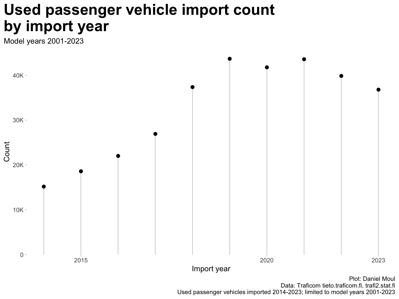
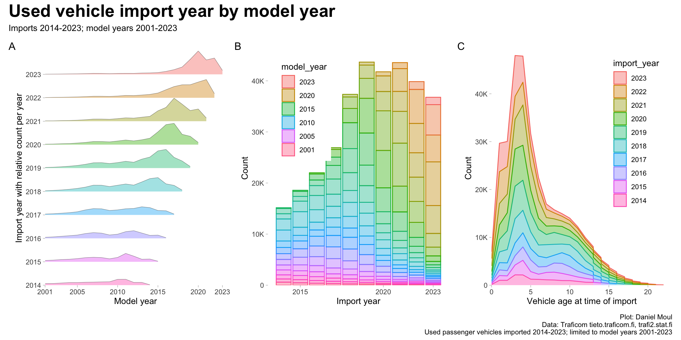
The data set includes used passenger vehicles imported during the years 2014-2023. I restrict the working set to vehicles of model years 2001+ and brands with more than 100 vehicles imported, resulting in model years 2001-2023, 86 brands with at least two imported vehicles, and 325632 vehicles over this time period. This slightly understates the total number of vehicle imported (see the long tails of older vehicles in 2014 and 2015 in panel A of Figure 6.2).

Show the code

dta |> 
  sample_n(10) |>
  gt() |>
  tab_header(md("**Sample rows of data: vehicle snapshot 2023-09-30**")) |>
  tab_options(table.font.size = 10)

Table 6.1: Sample used vehicle data - primary data fields

Sample rows of data: vehicle snapshot 2023-09-30
brand	model_year	power_train	import_year	n	n_brand_model_year	n_brand_all_years
Alfa Romeo	2018	Diesel	2021	13	67	507
Audi	2017	Petrol	2018	27	1916	24067
Audi	2001	Diesel	2014	11	173	24067
Citroen	2007	Diesel	2023	1	93	1215
BMW	2019	Petrol/Electricity (plug-in hybrid)	2021	1	1938	46239
Chevrolet	2004	Petrol/Ethanol	2018	1	25	922
VW	2010	Petrol/CNG	2015	4	1131	29949
Nissan	2013	Petrol	2021	3	127	3038
Opel	2012	Petrol/CNG	2020	1	549	2866
Suzuki	2021	Petrol/Electricity (plug-in hybrid)	2022	5	24	953

6.1 All brands

Show the code

dta_working_set |>
  summarize(count = sum(n),
            .by = import_year) |>
  ggplot() +
  geom_segment(aes(x = import_year, xend = import_year,
                   y = 0, yend = count),
               linewidth = 0.1) +
  geom_point(aes(import_year, count), size = 2) +
  scale_x_continuous(breaks = my_breaks$model_year) +
  scale_y_continuous(labels = label_number(scale_cut = cut_short_scale()),
                     expand = expansion(mult = c(0, 0.05))) +
  expand_limits(y = 0) +
  labs(
    title = "Used passenger vehicle import count\nby import year", 
    subtitle = glue("Model years {model_year_range}"),
    x = "Import year",
    y = "Count",
    caption = my_caption
  )

Figure 6.1: Used passenger vehicles imported to Finland

The most popular age for imported vehicles is four or five years old (Figure 6.2 panel A, panel C). At the same time, the yearly number of imports has been trending upwards since the first import year in this data set. Combining these trends: the record years are 2019 and 2021 (panel B).

Show the code

p1 <- dta_working_set |>
  mutate(import_year = factor(import_year)) |>
  summarize(n = sum(n),
            .by = c(import_year, model_year)
            ) |>
  ggplot() +
  geom_density_ridges(aes(x = model_year,
                          y = import_year, 
                          height = n,
                          group = import_year,
                          fill = import_year),
                      stat = "identity", scale = 1,
                      linewidth = 0.1, alpha = 0.4,
                      show.legend = FALSE) +
  scale_x_continuous(breaks = my_breaks$model_year,
                     expand = expansion(mult = c(0, 0.02))) +
  scale_y_discrete(expand = expansion(mult = c(0, 0.0))) +
  scale_fill_hue(direction = -1) +
  labs(
    x = "Model year",
    y = "Import year with relative count per year",
    tag = "A"
  )

p2 <- dta_working_set |>
  summarize(n = sum(n),
            .by = c(import_year, model_year)
            ) |>
  mutate(model_year = fct_rev(factor(model_year))) |>
  ggplot() +
  geom_col(aes(x = import_year,
               y = n,
               color = model_year,
               fill = model_year),
           alpha = 0.4) +
  scale_x_continuous(breaks = my_breaks$model_year) +
  scale_y_continuous(labels = label_number(scale_cut = cut_short_scale()),
                     expand = expansion(mult = c(0, 0.05))) +
  scale_color_discrete(breaks = c(2001, 2005, 2010, 2015, 2020, 2023)) +
  scale_fill_discrete(breaks = c(2001, 2005, 2010, 2015, 2020, 2023)) +
  guides(color = guide_legend(reverse=TRUE)) + 
  guides(fill = guide_legend(reverse=TRUE)) +
  theme(legend.position = c(0.2, 0.75)) +
  labs(
    x = "Import year",
    y = "Count",
    tag = "B"
  )

p3 <- dta_working_set |>
  mutate(vehicle_age = import_year - model_year,
         import_year = fct_rev(factor(import_year))) |>
  summarize(n = sum(n),
            .by = c(import_year, vehicle_age)
            ) |>
  arrange(import_year) |>
  ggplot() +
  geom_area(aes(x = vehicle_age,
                y = n,
                group = import_year,
                color = import_year,
                fill = import_year),
            alpha = 0.4) +
  scale_x_continuous(expand = expansion(mult = c(0, 0.05))) +
  scale_y_continuous(labels = label_number(scale_cut = cut_short_scale()),
                     expand = expansion(mult = c(0, 0.02))) +
  theme(legend.position = c(0.8, 0.65)) +
  labs(
    x = "Vehicle age at time of import",
    y = "Count",
    tag = "C"
  )

p1 + p2 + p3 +
  plot_annotation(
    title = "Used vehicle import year by model year",
    subtitle = glue("Imports 2014-2023; model years {model_year_range}"),
    caption = my_caption
  )

Figure 6.2: Used passenger vehicles imported to Finland - by import year and model year

6.2 Brands

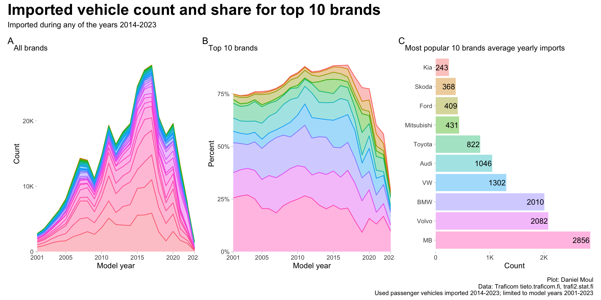
The most popular used car import brands includes most of the same brands as the top brands in the inspection data Figure 1.6, however the ranking is different: Mercedes-Benz, Volvo, and BMW have higher shares, and VW and Toyota have lower shares (compare with Figure 1.6)

Show the code

data_for_plot <- dta_by_brand_power_train |>
  summarize(count = sum(count),
            .by = c(model_year, brand)
            ) |>
  mutate(brand = fct_lump_min(brand, min = 100, w = count)) |>
  summarize(count = sum(count),
            .by = c(model_year, brand)
            ) |>
  mutate(brand = fct_reorder(brand, count, sum))

p1 <- data_for_plot |>
  ggplot() +
  geom_area(aes(model_year, count, color = brand, fill = brand),
            show.legend = FALSE,
            alpha = 0.4) +
  scale_x_continuous(breaks = my_breaks$model_year,
                     expand = expansion(mult = c(0, 0))) +
  scale_y_continuous(labels = label_number(scale_cut = cut_short_scale()),
                     expand = expansion(mult = c(0, 0.05))) +
  expand_limits(y = 0) +
  labs(
    subtitle = "All brands",
    x = "Model year",
    y = "Count",
    tag = "A"
  )

data_for_plot_v2 <- data_for_plot |>
  mutate(pct_count_model_year = count / sum(count),
         .by = model_year) |>
  mutate(count_brand_all_years = sum(count),
         .by = brand) |>
  mutate(brand = fct_lump(brand, n = brand_cutoff_n, w = count_brand_all_years)) |>
  reframe(count = sum(count),
          pct_count_model_year = sum(pct_count_model_year),
          .by = c(model_year, brand)
            ) |>
  mutate(count_brand_all_years = sum(count),
         .by = brand) |>
  mutate(brand = fct_reorder(brand, count, sum))

data_for_plot_labels <- data_for_plot_v2 |>
  filter(model_year == max_model_year)


p2 <- data_for_plot_v2 |>
  filter(brand != "Other") |>
  droplevels() |>
  ggplot() +
  geom_area(aes(model_year, pct_count_model_year, color = brand, fill = brand),
            show.legend = FALSE,
            na.rm = TRUE,
            alpha = 0.4) +
  scale_x_continuous(breaks = my_breaks$model_year,
                     expand = expansion(mult = c(0, 0))) +
  scale_y_continuous(labels = label_percent(),
                     expand = expansion(mult = c(0, 0.05))) +
  expand_limits(y = 0) +
  labs(
    subtitle = glue("Top {brand_cutoff_n} brands"),
    x = "Model year",
    y = "Percent",
    tag = "B"
  )

p3 <- data_for_plot_v2 |>
  mutate(avg_import_count_brand = count_brand_all_years / n(),
         .by = brand) |>
  filter(brand != "Other") |>
  distinct(brand, .keep_all = TRUE) |>
  mutate(brand = fct_rev(brand),
         label_count_brand_all_years = glue("{round(avg_import_count_brand)}"),
         ) |>
  ggplot(aes(avg_import_count_brand, brand, fill = brand)) + #pct_count_model_year
  geom_col(na.rm = TRUE, show.legend = FALSE, alpha = 0.4) +
  geom_text(aes(label =  label_count_brand_all_years),
            hjust = 1, nudge_x = -10) + #, nudge_x = -1
  scale_x_continuous(labels = label_number(scale_cut = cut_short_scale()),
                     expand = expansion(mult = c(0, 0.02))) +
  scale_fill_hue(direction = -1) +
  expand_limits(x = 0) +
  theme(panel.border = element_blank()) +
  labs(
    subtitle = glue("Most popular {brand_cutoff_n} brands average yearly imports"),
    x = "Count",
    y = NULL,
    tag = "C"
  )

p1 + p2 + p3 + 
  plot_annotation(
    title = glue("Imported vehicle count and share for top {brand_cutoff_n} brands"),
    subtitle = "Imported during any of the years 2014-2023",
    caption = my_caption
  )

Figure 6.3: Used Vehicle imports: count and share for 10 most popular brands

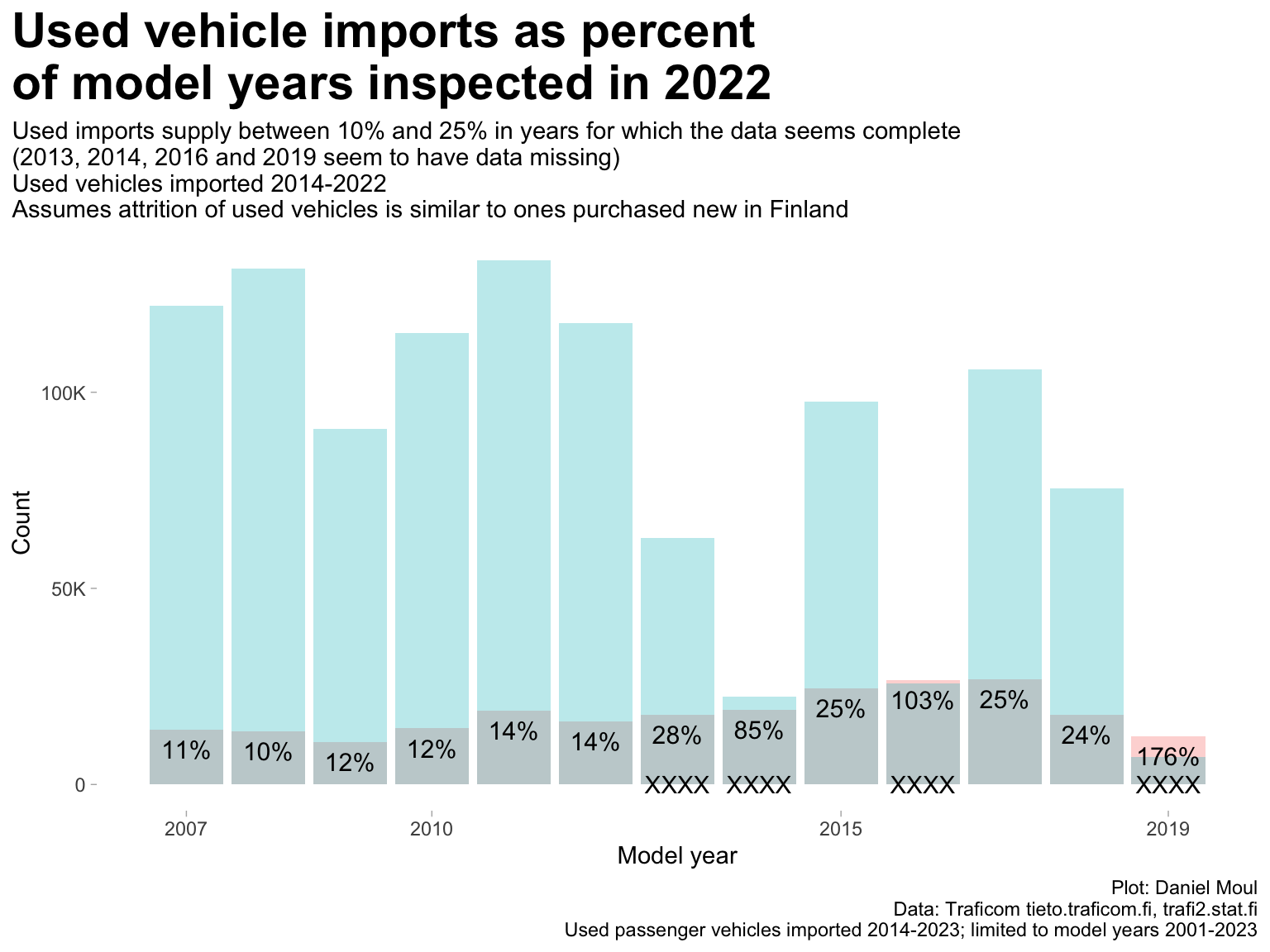
6.3 Used vehicle imports as percent of model year inspected

Show the code

dta_imported_yearly_count <- dta_working_set |>
  filter(import_year <= 2022) |> # don't include imports after the 2022 inspection year
  count(model_year, wt = n, name = "import_count")

dta_imported_inspected <- dta_imported_yearly_count |>
  left_join(dta_inspections_yearly_count,
            by = join_by(model_year)) |>
  filter(!is.na(inspection_count)) |>
  mutate(pct = import_count / inspection_count)

After four or five years, used vehicle imports supply up to about a quarter of the passenger vehicles on the road in Finland for any model year (Figure 6.4). Percentages prior to 2014 likely are under counts, since the data set does not include vehicles imported during years before 2014.

Show the code

data_for_plot <- dta_imported_inspected |>
  pivot_longer(cols = c(import_count, inspection_count),
               names_to = "metric",
               values_to = "value")

min_model_year_plot <- min(data_for_plot$model_year)
max_model_year_plot <- max(data_for_plot$model_year)

plot_breaks <- data_for_plot |>
  distinct(model_year) |>
  filter(model_year %in%  c(min_model_year_plot, max_model_year_plot) |
           model_year %% 5 == 0)

data_for_plot |>
  ggplot() +
  geom_col(aes(model_year, 
               value,
               fill = metric
               ),
           position = position_identity(),
           #position = position_dodge(),
           show.legend = FALSE,
           na.rm = TRUE, alpha = 0.3) +
  geom_text(aes(model_year, 
               ifelse(metric %in% c("inspection_count"),
                                   value * pct,
                                   NA),
               label = percent(pct, accuracy = 1)
               ),
            na.rm = TRUE, hjust = 0.5, nudge_y = -5000, size = 4
            ) +
  geom_text(data = tibble(model_year = c(2013, 2014, 2016, 2019),
                          value = 100,
                          label = "XXXX"),
            aes(model_year, value, label = label)) +
  scale_x_continuous(breaks = plot_breaks$model_year) +
  scale_y_continuous(labels = label_number(scale_cut = cut_short_scale())) +
  labs(
    title = "Used vehicle imports as percent\nof model years inspected in 2022",
    subtitle = glue("Used imports supply between 10% and 25% in years for which the data seems complete",
                    "\n(2013, 2014, 2016 and 2019 seem to have data missing)",
                    "\nUsed vehicles imported 2014-2022",
                    "\nAssumes attrition of used vehicles is similar to ones purchased new in Finland"),
    x = "Model year",
    y = "Count",
    fill = NULL,
    caption = my_caption
  )

Figure 6.4: Imports of model years as percent of all model years inspected in 2022