5  Changing power train mix

Finland, as part of the European union, have committed to zero-emission new cars and vans by 2035¹

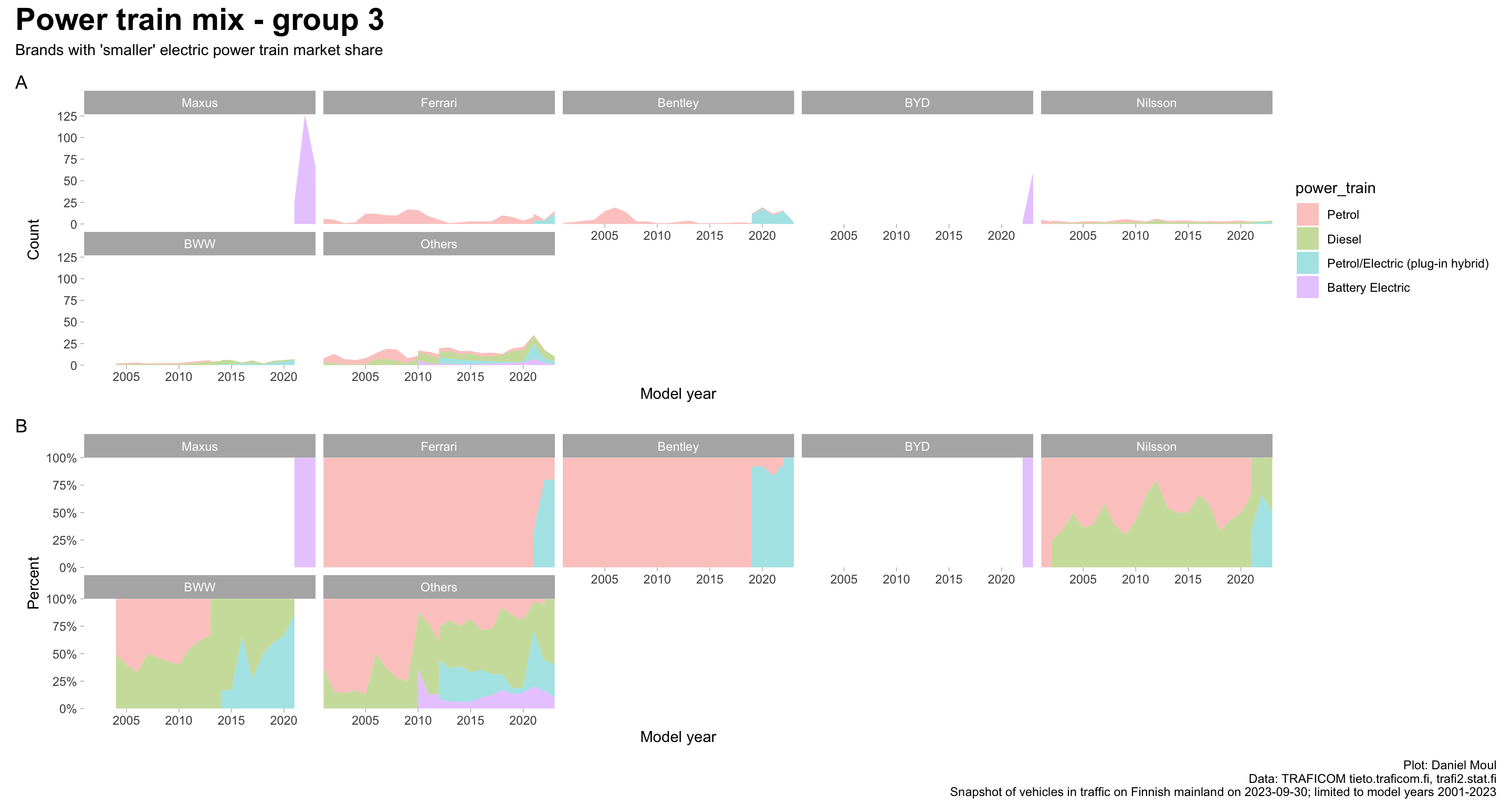
International trends towards lower-emissions vehicles are already visible in a snapshot of passenger vehicles in traffic in mainland Finland on 2023-09-30 (even with the biases associated with this approach to data collection which are noted in Section A.2). After restricting the data set to model years 2001-2023, it includes 71 brands and 8 types of power train. See Appendix C Power train mix by brand.

Key observations:

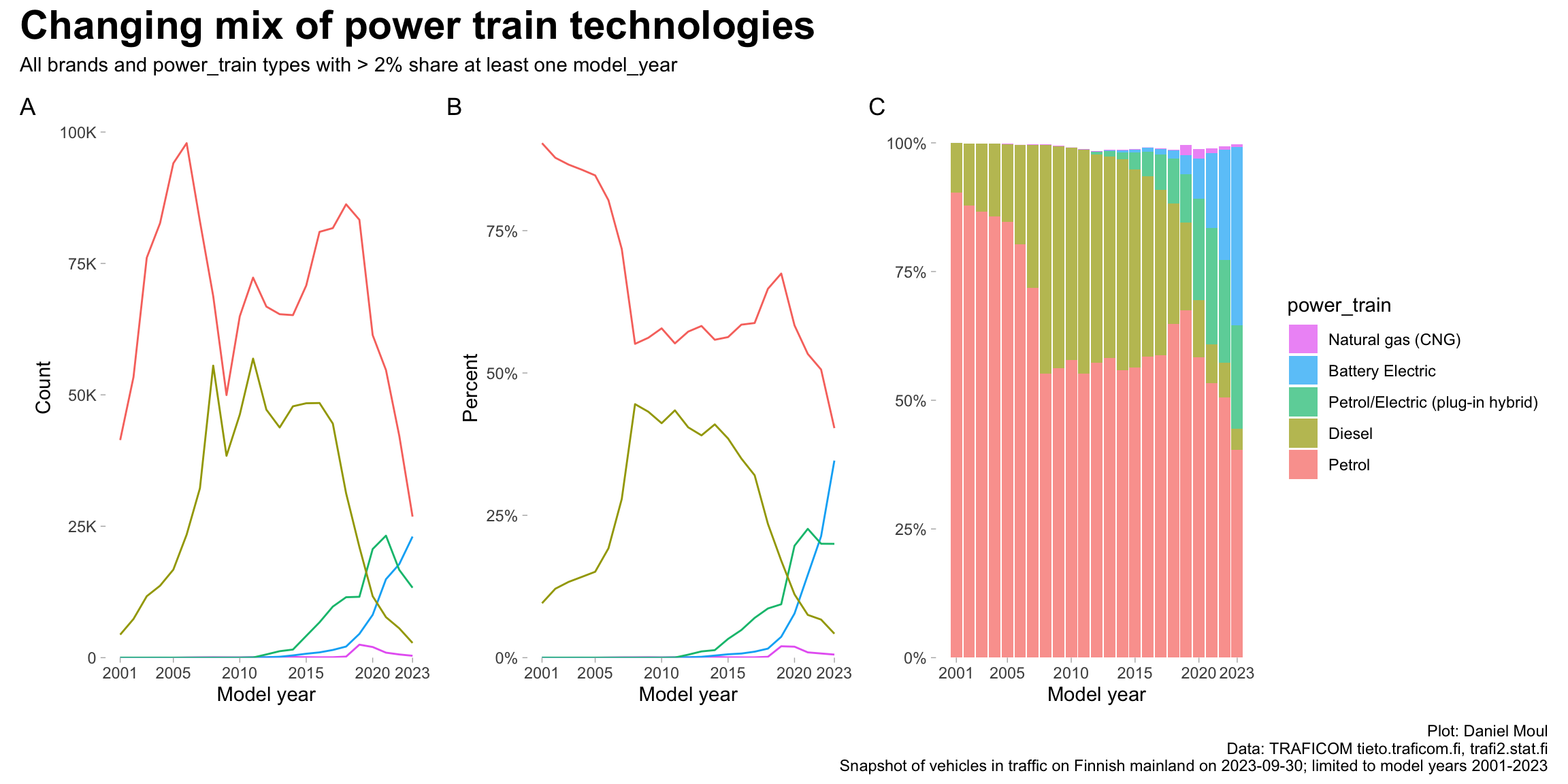
• Diesel power trains largely have finished their run (Figure 5.2)
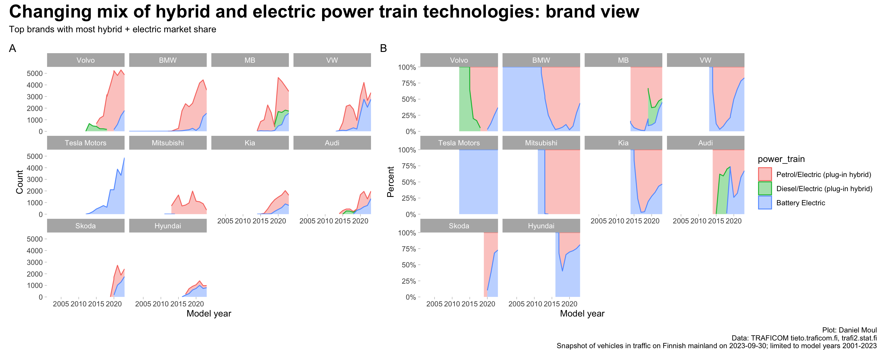
• Petrol-hybrid electric (and to a much lesser extent, diesel-hybrid electric) seem to be transitional technologies on the way to battery electric (Figure 5.2 and Figure 5.8)
• Some brands have effectively transitioned sales to hybrid and battery electric vehicles (Volvo, Mercedes-Benz, BMW and Audi) while others remain very dependent on petrol sales (especially Toyota though it is in the top 10 brands with most hybrid and battery electric vehicles) (Figure 5.2, Figure 5.8, Figure 5.9)
• New brands are taking advantage of the move to battery electric: Tesla opened an early lead and remains market share leader. Other brands are growing from small numbers: Swedish Polestar (owned by Volvo), and Chinese brands BYD, Magnus, and MG. (Figure 5.11, Figure 5.12, Figure 5.13)

Below I refer to “hybrid” to mean petrol/electric hybrid and/or diesel/electric hybrid. I use “Electric” to refer to hybrid or battery electric (BEV). Where I refer exclusively to battery electric I make that clear.

TODO: Can I find more info on what “in traffic” means?

Show the code

##| column: page-right

dta |> 
  select(-area) |>
  filter(n > 0) |>
  sample_n(10) |>
  gt() |>
  tab_header(md("**Sample rows of data: vehicle snapshot 2023-09-30**")) |>
  tab_options(table.font.size = 10)

Table 5.1: Sample data - primary data fields

Sample rows of data: vehicle snapshot 2023-09-30
model_year	brand	power_train	n
2005	Bentley	Petrol	15
2003	Volvo	Petrol/CNG	43
2015	Mini	Diesel	44
2015	Fiat	Petrol/CNG	1
2014	Mitsubishi	Petrol/Electric (plug-in hybrid)	1186
2014	Others	Battery Electric	1
2011	Renault	Petrol/Ethanol	29
2015	Kia	Petrol	5206
2010	Ford	Petrol/Ethanol	331
2022	Renault	Petrol	888

5.1 All brands

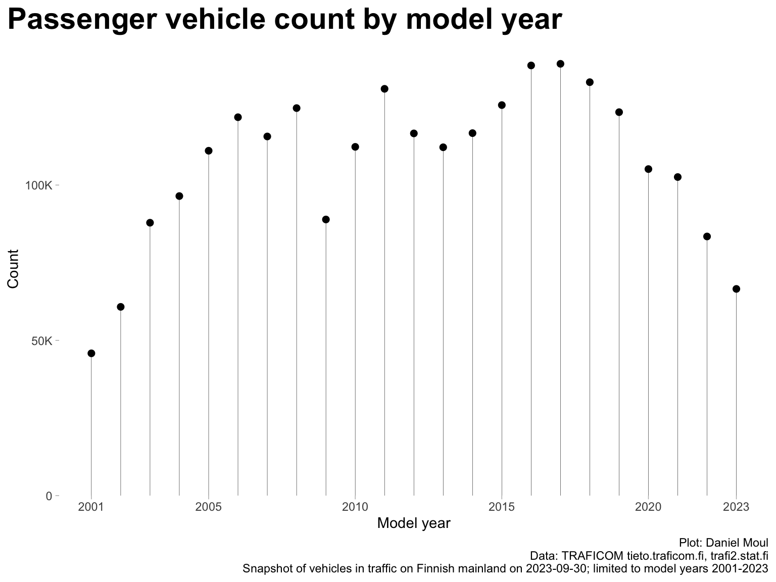
In Figure 5.1 there is surprising variability in the count of vehicles by model_year. Why?

• I assume 2009 can be explained by fewer vehicles being purchased during the global financial crisis.
• Drops starting in 2020 are probably due to the COVID-19 pandemic and resulting supply chain constraints as well as use car imports being older models (the most common age of used vehicle imports is four or five years; see Figure 6.2 panel C).
• The relatively low count in 2023 is not a surprise: the data is a snapshot at 2023-09-30, so it reflects only about three quarters of sales (“about”, since some new cars of the latest model years come to market late in the prior calendar year, and some new cars are not sold until the calendar year after the model year).
• I assume the declining counts before 2016 are the result of the normal attrition of passenger vehicles over time: accidents, mechanical failures, rust, general decay, and owners purchasing newer cars as their “old” vehicles age and become less reliable.

Show the code

dta_by_power_train |>
  summarize(count = sum(count),
            .by = model_year) |>
  ggplot() +
  geom_segment(aes(x = model_year, xend = model_year, 
                   y = 0, yend = count),
               linewidth = 0.1) +
  geom_point(aes(model_year, count), size = 2) +
  scale_x_continuous(breaks = my_breaks$model_year) +
  scale_y_continuous(labels = label_number(scale_cut = cut_short_scale()),
                     expand = expansion(mult = c(0, 0.05))) +
  expand_limits(y = 0) +
  labs(
    title = "Passenger vehicle count by model year",
    x = "Model year",
    y = "Count",
    caption = my_caption
  )

Figure 5.1: Passenger vehicles in traffice in Finland on 2023-09-30

Looking at the market share of major power train technologies in Figure 5.2 the macro trends are interesting: diesel passenger vehicles displaced a large portion of petrol engines starting in 2005 and then went into steep decline by 2017 (the VW diesel emissions defeat device scandal became public in late 2015 [BBC News]). Petrol-hybrid and battery electric power trains first replaced diesel then started taking market share from petrol power trains. It seems likely to me that these trends can be found in many other countries.

Show the code

data_for_plot <- dta_by_power_train |>
  filter(any(pct > 0.02),
         .by = "power_train")

p1 <- data_for_plot |>
  ggplot() +
  geom_line(aes(model_year, count, color = power_train, group = power_train),
            show.legend = FALSE) +
  scale_x_continuous(breaks = my_breaks$model_year) +
  scale_y_continuous(labels = label_number(scale_cut = cut_short_scale()),
                     expand = expansion(mult = c(0, 0.05))) +
  scale_color_hue(direction = -1) +
  labs(
    x = "Model year",
    y = "Count",
    tag = "A"
  )

p2 <- data_for_plot |>
  ggplot() +
  geom_line(aes(model_year, pct, color = power_train, group = power_train),
            show.legend = FALSE) +
  scale_x_continuous(breaks = my_breaks$model_year) +
  scale_y_continuous(labels = label_percent(),
                     expand = expansion(mult = c(0, 0.05))) +
  scale_color_hue(direction = -1) +
  labs(
    x = "Model year",
    y = "Percent",
    tag = "B"
  )

p3 <- data_for_plot |>
  ggplot() +
  geom_col(aes(model_year, pct, fill = power_train, group = power_train),
           alpha = 0.7) +
  scale_x_continuous(breaks = my_breaks$model_year) +
  scale_y_continuous(labels = label_percent(),
                     expand = expansion(mult = c(0, 0.05))) +
  scale_fill_hue(direction = -1) +
  labs(
    x = "Model year",
    y = NULL,
    tag = "C"
  )

p1 + p2 + p3 +
  plot_annotation(
    title = "Changing mix of power train technologies",
    subtitle = "All brands and power_train types with > 2% share at least one model_year",
    caption = my_caption
  )

Figure 5.2: Changing power train mix

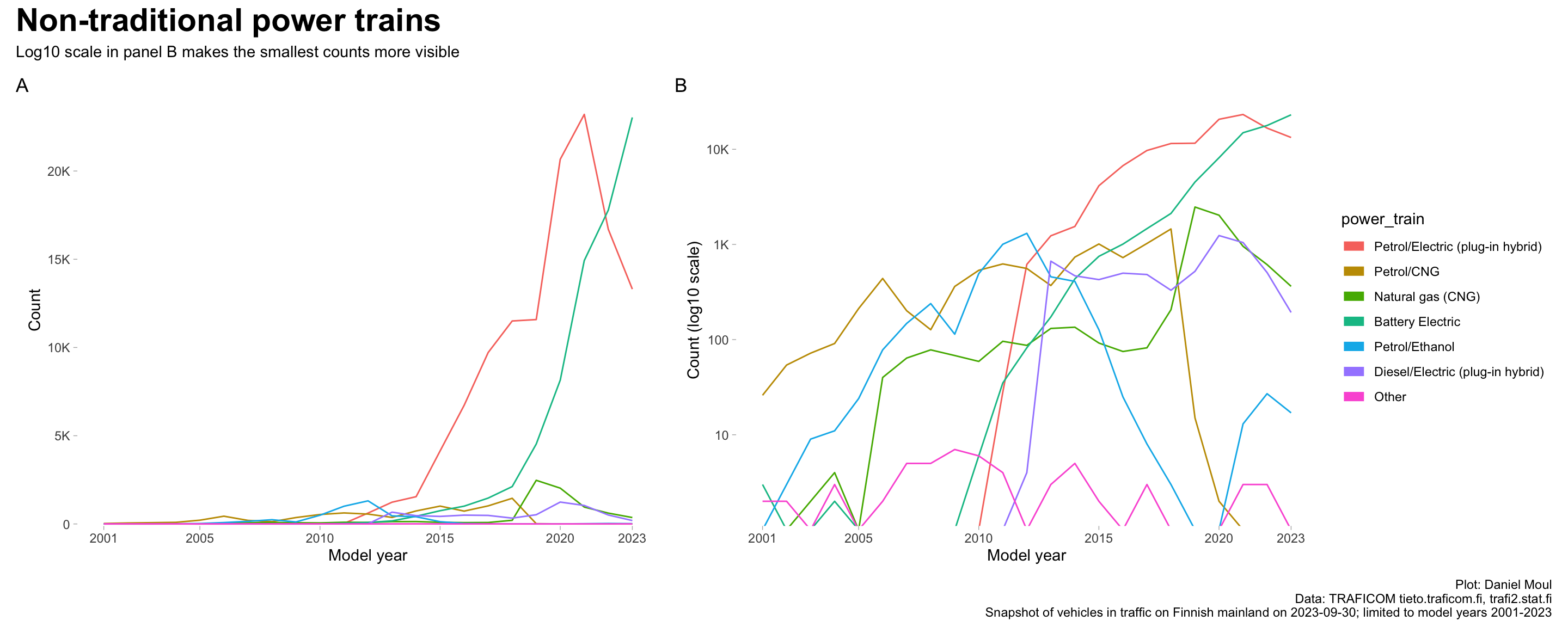
If we define petrol and diesel power trains as “traditional” and consider only the “non-traditional” power trains, the rise of petrol hybrid-electric (“Petrol/Electric”) followed a few years later by battery electric vehicles becomes visible in Figure 5.3. At least in Finland, the petrol hybrid seems to be a transitional technology on the path to battery electric. It’s too soon to say whether there is an enduring place for petrol hybrids (if anywhere, it probably would be in the north where it gets very cold (batteries operate with lower efficiency in very cold weather) and/or in rural areas where electric charging infrastructure may be less available and people need to drive farther).

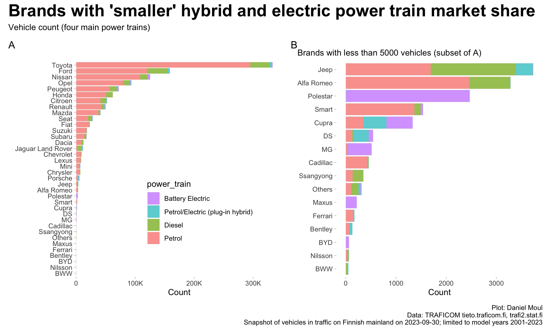
None of the other types of power trains gained momentum: less than about 2000 vehicles of any of these types were sold in any model year.

Show the code

dta_by_power_train_not_traditional <- dta_by_power_train |>
  filter(!power_train %in% c("Petrol", "Diesel")) |>
  mutate(power_train = fct_reorder(power_train, -count),
         count = if_else(count == 0,
                         1,
                         count)
         )

p1 <- dta_by_power_train_not_traditional |>
  ggplot() +
  geom_line(aes(model_year, count, color = power_train, group = power_train),
            show.legend = FALSE) +
  scale_x_continuous(breaks = my_breaks$model_year) +
  scale_y_continuous(labels = label_number(scale_cut = cut_short_scale()),
                     expand = expansion(mult = c(0.005, 0.05))) +
  guides(color = guide_legend(override.aes = list(linewidth = 3),
                              reverse = FALSE)) +
  labs(
    x = "Model year",
    y = "Count",
    tag = "A"
  )

p2 <- dta_by_power_train_not_traditional |>
  filter(count > 0) |>
  ggplot() +
  geom_line(aes(model_year, count, color = power_train, group = power_train),
            show.legend = TRUE) +
  scale_x_continuous(breaks = my_breaks$model_year) +
  scale_y_log10(labels = label_number(scale_cut = cut_short_scale()),
                expand = expansion(mult = c(0, 0.05))) +
  coord_cartesian(ylim = c(1.1, NA)) +
  guides(color = guide_legend(override.aes = list(linewidth = 3),
                              reverse = FALSE)) +
  labs(
    x = "Model year",
    y = "Count (log10 scale)",
    tag = "B"
  )

p1 + p2 + 
  plot_annotation(
    title = "Non-traditional power trains",
    subtitle = "Log10 scale in panel B makes the smallest counts more visible",
    caption = my_caption
  )

Figure 5.3: Non-traditional power trains

5.2 By brands

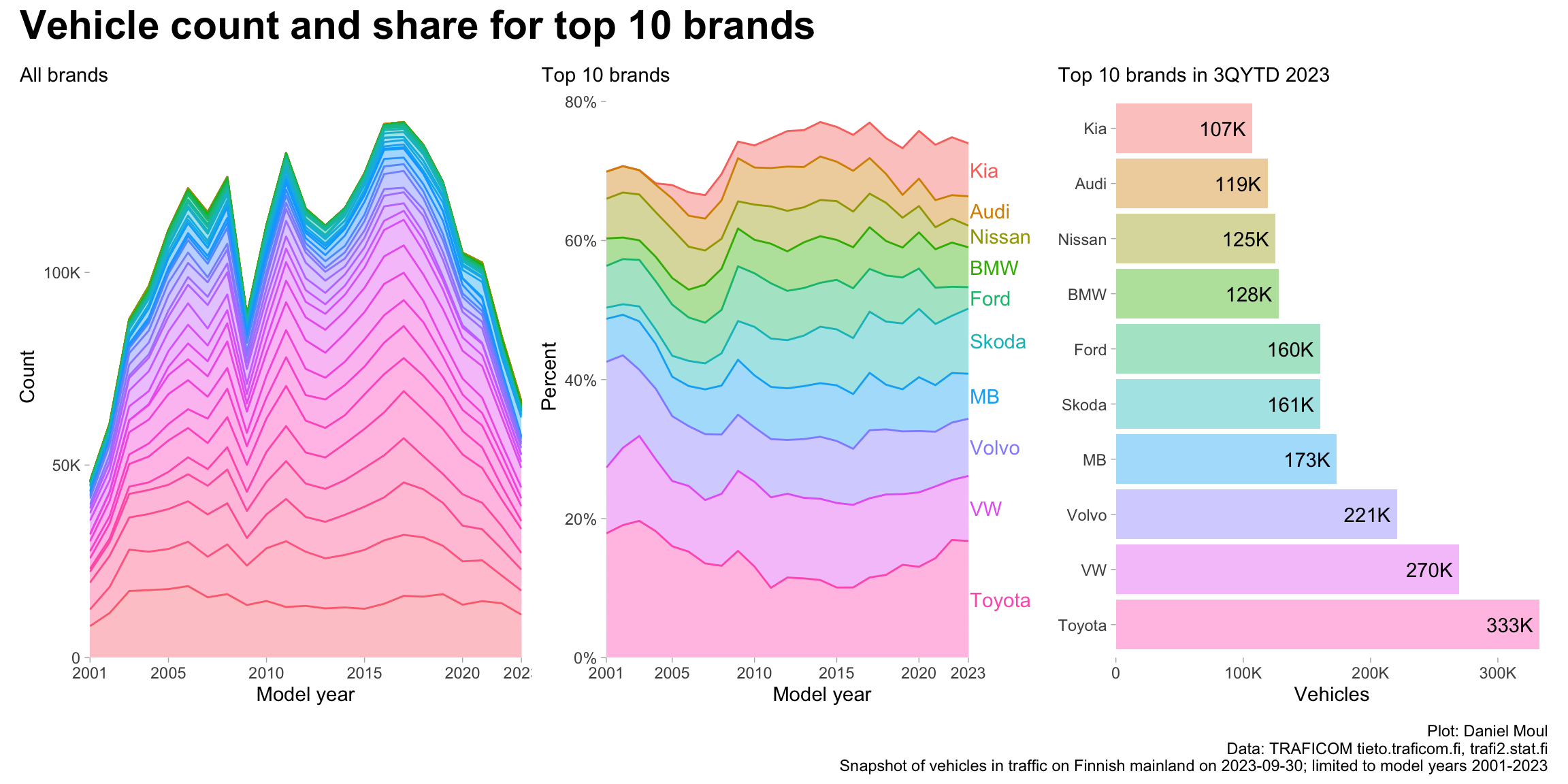
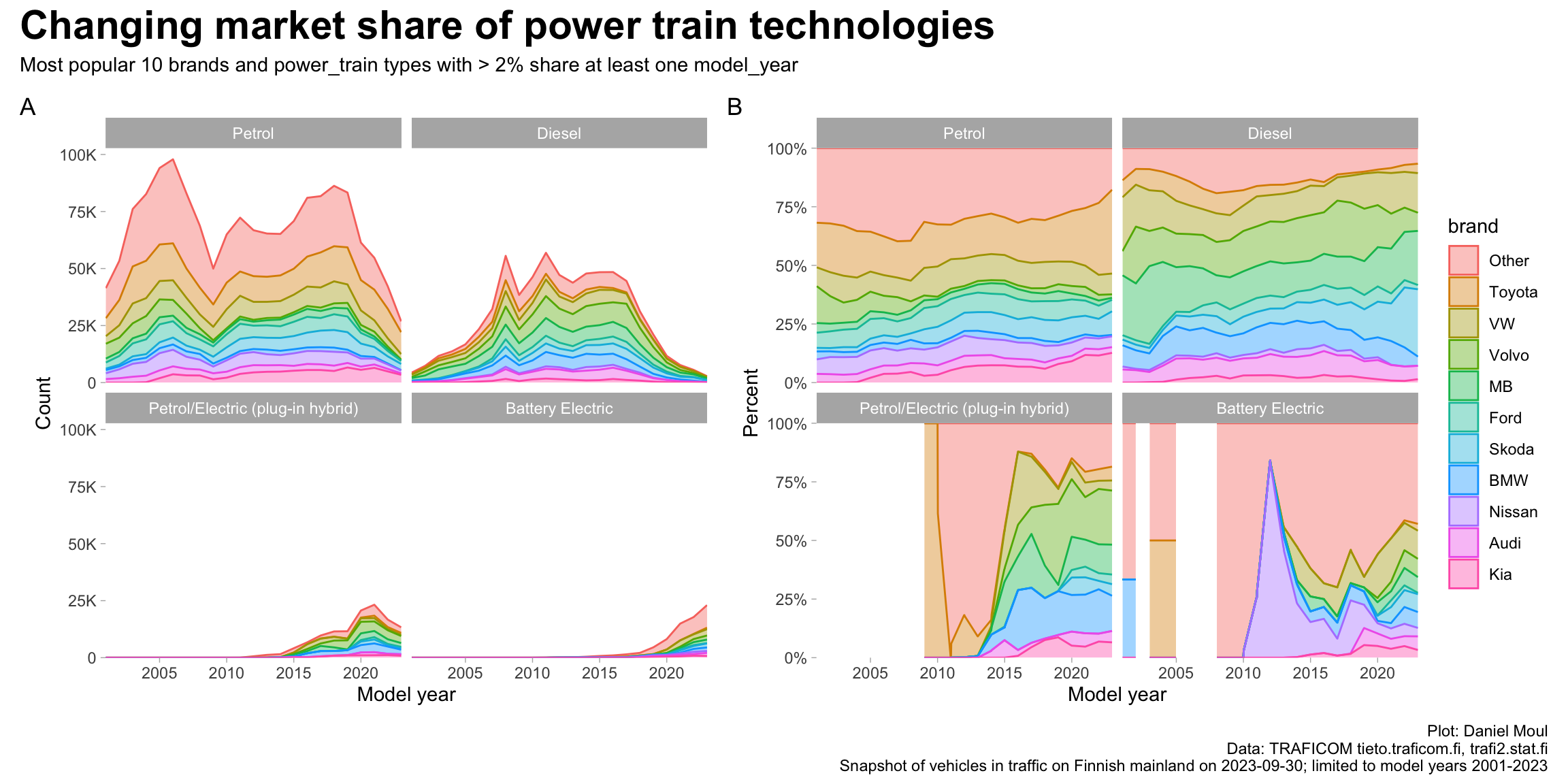
While there are 71 brands in the data, the ten most popular brands have supplied about three quarters of the vehicles for more than a decade (Figure 5.4 panel B). There are three VW brands in the top ten: VW, Skoda, and Audi.

Show the code

data_for_plot <- dta_by_brand_power_train |>
  summarize(count = sum(count),
            .by = c(model_year, brand)
            ) |>
  mutate(brand = fct_lump_min(brand, min = 100, w = count)) |>
  summarize(count = sum(count),
            .by = c(model_year, brand)
            ) |>
  mutate(brand = fct_reorder(brand, count, sum))

p1 <- data_for_plot |>
  ggplot() +
  geom_area(aes(model_year, count, color = brand, fill = brand),
            show.legend = FALSE,
            alpha = 0.4) +
  scale_x_continuous(breaks = my_breaks$model_year,
                     expand = expansion(mult = c(0, 0))) +
  scale_y_continuous(labels = label_number(scale_cut = cut_short_scale()),
                     expand = expansion(mult = c(0, 0.05))) +
  expand_limits(y = 0) +
  labs(
    subtitle = "All brands",
    x = "Model year",
    y = "Count"
  )

data_for_plot_v2 <- data_for_plot |>
  mutate(pct_count_model_year = count / sum(count),
         .by = model_year) |>
  mutate(count_brand_all_years = sum(count),
         .by = brand) |>
  mutate(brand = fct_lump(brand, n = brand_cutoff_n, w = count_brand_all_years)) |>
  reframe(count = sum(count),
          pct_count_model_year = sum(pct_count_model_year),
          .by = c(model_year, brand)
            ) |>
  mutate(count_brand_all_years = sum(count),
         .by = brand) |>
  mutate(brand = fct_reorder(brand, count, sum))

data_for_plot_labels <- data_for_plot_v2 |>
  filter(model_year == max_model_year)


p2 <- data_for_plot_v2 |>
  filter(brand != "Other") |>
  droplevels() |>
  ggplot() +
  geom_area(aes(model_year, pct_count_model_year, color = brand, fill = brand),
            show.legend = FALSE,
            na.rm = TRUE,
            alpha = 0.4) +
  geom_text(
    aes(x = if_else(model_year == max_model_year,
                    model_year + 0.1,
                    NA), 
        y = if_else(model_year == max_model_year,
                    pct_count_model_year, 
                    NA),
        color = brand, 
        label = brand),
        na.rm = TRUE,
        show.legend = FALSE,
    position = position_stack(vjust = 0.5),
    hjust = 0) +
  scale_x_continuous(breaks = my_breaks$model_year,
                     expand = expansion(mult = c(0, 0.05))) +
  scale_y_continuous(labels = label_percent(),
                     expand = expansion(mult = c(0, 0.05))) +
  expand_limits(y = 0) +
  coord_cartesian(xlim = c(NA, max_model_year + 3)) +
  labs(
    subtitle = glue("Top {brand_cutoff_n} brands"),
    x = "Model year",
    y = "Percent"
  )

p3 <- data_for_plot_labels |>
  filter(brand != "Other") |>
  mutate(brand = fct_rev(brand),
         label_count_brand_all_years = glue("{round(count_brand_all_years / 1000)}K")) |>
  ggplot(aes(count_brand_all_years, brand, fill = brand)) +
  geom_col(na.rm = TRUE, show.legend = FALSE, alpha = 0.4) +
  geom_text(aes(label =  label_count_brand_all_years),
            hjust = 1, nudge_x = -5000) + #
  scale_x_continuous(labels = label_number(scale_cut = cut_short_scale()),
                     expand = expansion(mult = c(0, 0.02))) +
  scale_fill_hue(direction = -1) +
  expand_limits(x = 0) +
  theme(panel.border = element_blank()) +
  labs(
    subtitle = glue("Top {brand_cutoff_n} brands in 3QYTD {max_model_year}"),
    x = "Vehicles",
    y = NULL
  )

p1 + p2 + p3 + 
  plot_annotation(
    title = glue("Vehicle count and share for top {brand_cutoff_n} brands"),
    caption = my_caption
  )

Figure 5.4: Vehicle count and share for 10 most popular brands

5.2.1 Changing market share

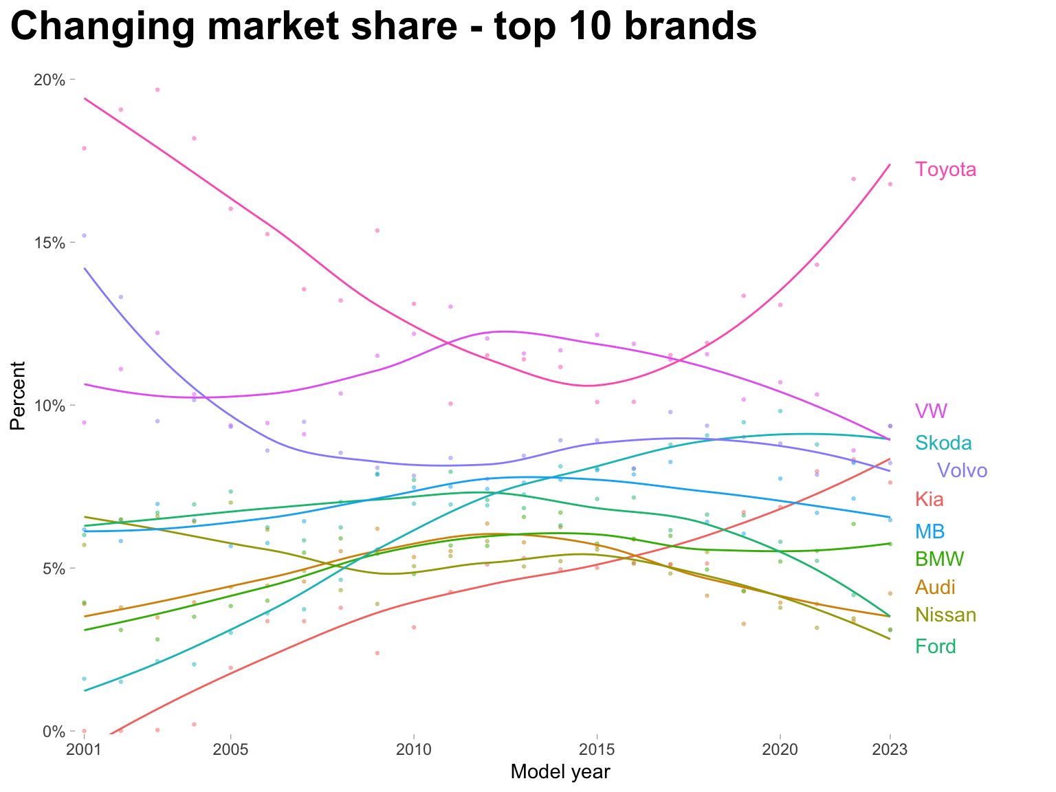
The vehicle snapshot on 2023-09-30 provides one source of data from which to build a view of changing passenger vehicle market share in Finland (Figure 5.5).

• Skoda and Kia have done a remarkable job growing market share over the last 20+ years.
• Toyota executed an impressive turn-around to restore their market-leading position over the last eight years.
• Market shares of VW, Audi, Nissan, and Ford are in significant multi-year decline.
• Market shares of Volvo, Mercedes-Benz, and BMW have been relatively stable over the last eight-to-ten years.

Show the code

data_for_plot_v2 |>
  filter(brand != "Other") |>
  droplevels() |>
  ggplot() +
  geom_point(aes(model_year, pct_count_model_year, color = brand, group = brand),
            show.legend = FALSE,
            na.rm = TRUE,
            size = 0.5,
            alpha = 0.4) +
  geom_smooth(aes(model_year, pct_count_model_year, color = brand, group = brand),
            show.legend = FALSE,
            na.rm = TRUE,
            linewidth = 0.5,
            se = FALSE, method = "loess", formula = 'y ~ x',
            alpha = 0.4) +
  geom_text_repel(
    aes(x = if_else(model_year == max_model_year,
                    model_year + 1,
                    NA), 
        y = if_else(model_year == max_model_year,
                    pct_count_model_year, 
                    NA),
        color = brand, 
        label = brand),
    na.rm = TRUE,
    show.legend = FALSE,
    xlim = c(max_model_year + 0.5, NA),
    hjust = 0) +
  scale_x_continuous(breaks = my_breaks$model_year,
                     expand = expansion(mult = c(0.01, 0.05))
                     ) +
  scale_y_continuous(labels = label_percent(),
                     expand = expansion(mult = c(0, 0.05))
                     ) +
  expand_limits(y = 0) +
  coord_cartesian(xlim = c(NA, max_model_year + 3),
                  ylim = c(-0.001, NA)) +
  theme(panel.border = element_blank()) +
  labs(
    title = glue("Changing market share - top {brand_cutoff_n} brands"),
    x = "Model year",
    y = "Percent"
  )

Figure 5.5: Changing market share of the most popular brands

Show the code

data_for_plot <- dta_by_brand_power_train |>
  filter(any(pct > 0.02),
         .by = "power_train") |>
  mutate(brand = fct_lump(brand, n = brand_cutoff_n, w = count)) |>
  summarize(count = sum(count),
          pct = sum(pct),
          .by = c(model_year, brand, power_train)) |>
  mutate(brand = fct_reorder(brand, -count, sum),
         power_train = fct_rev(power_train))

p1 <- data_for_plot |>
  ggplot() +
  geom_area(aes(model_year, count, color = brand, fill = brand, group = brand),
            show.legend = FALSE,
            alpha = 0.4) +
  scale_x_continuous(breaks = my_breaks_five_yearly$model_year,
                     expand = expansion(mult = c(0, 0))) +
  scale_y_continuous(labels = label_number(scale_cut = cut_short_scale()),
                     expand = expansion(mult = c(0, 0.05))) +
  facet_wrap( ~power_train) +
  labs(
    x = "Model year",
    y = "Count",
    tag = "A"
  )

p2 <- data_for_plot |>
  ggplot() +
  geom_area(aes(model_year, count, color = brand, fill = brand, group = brand),
            position = position_fill(),
            show.legend = TRUE,
            alpha = 0.4) +
  scale_x_continuous(breaks = my_breaks_five_yearly$model_year,
                     expand = expansion(mult = c(0, 0))) +
  scale_y_continuous(labels = label_percent(),
                     expand = expansion(mult = c(0, 0))) +
  facet_wrap( ~power_train) +
  labs(
    x = "Model year",
    y = "Percent",
    tag = "B"
  )

p1 + p2 +
  plot_annotation(
    title = "Changing market share of power train technologies",
    subtitle = glue("Most popular {brand_cutoff_n} brands and power_train types with > 2% share at least one model_year"),
    caption = my_caption
  )

Figure 5.6: Changing power train market share

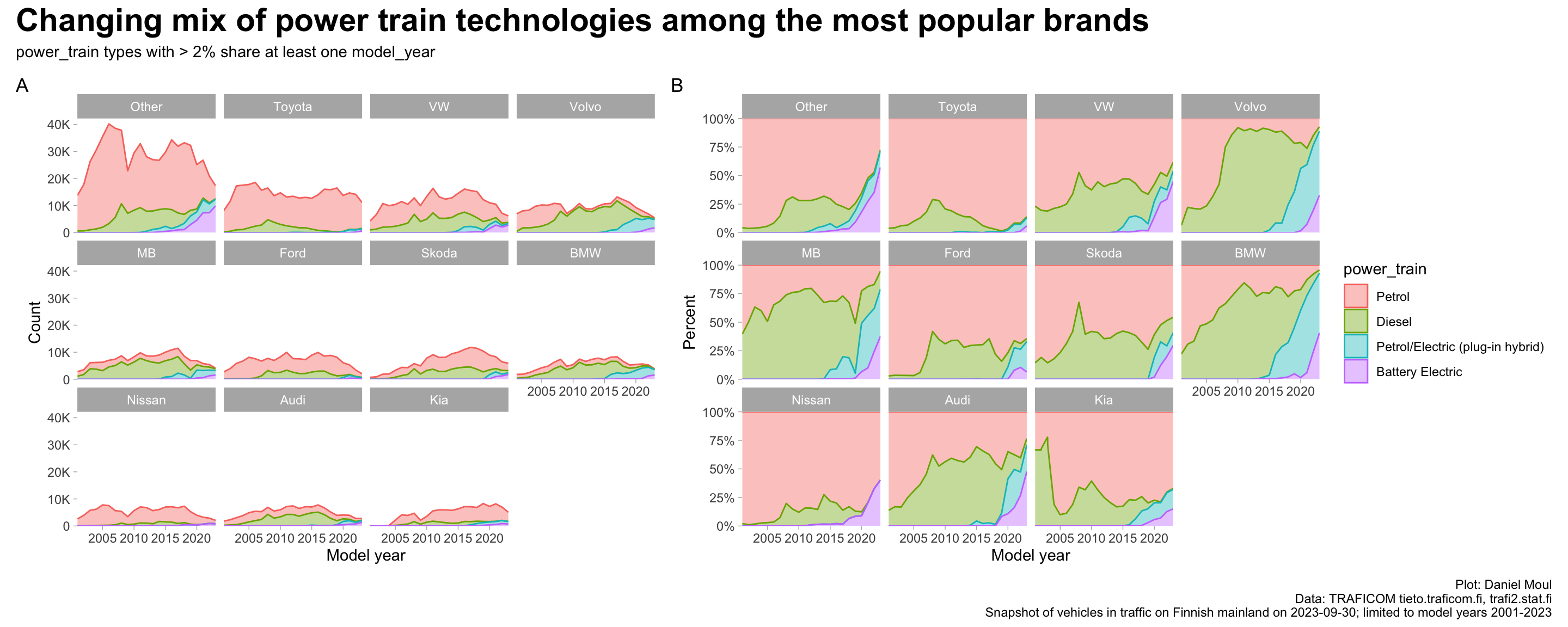
It’s worth looking at brand trends related to electrically powered vehicles. In Figure 5.7 it’s impressive to see the degree to which a set of market share leaders (Volvo, Mercedes-Benz, BMW and Audi) transitioned from large-majority petrol and/or diesel power as recently as 2017 to well over 80% battery electric or petrol hybrid in the first three quarters of 2023.

Toyota on the other hand, despite offering hybrid power trains for many models, is highly concentrated in petrol power. Executives there must be nervous that their market share could collapse if new car buyers’ sentiment turns strongly against petrol vehicles without transferring their Toyota brand preferences to Toyota’s hybrid or electric power trains.

To a lesser extent Ford, Skoda, Nisan and Kia remain dependent on petrol and diesel sales, however they all seem to be experiencing growing credible electric and/or petrol-electric momentum.

Show the code

data_for_plot <- dta_by_brand_power_train |>
  filter(any(pct > 0.02),
         .by = "power_train") |>
  mutate(brand = fct_lump(brand, n = brand_cutoff_n, w = count)) |>
  summarize(count = sum(count),
          pct = sum(pct),
          .by = c(model_year, brand, power_train)) |>
  mutate(brand = fct_reorder(brand, -count, sum),
         power_train = fct_rev(power_train))

p1 <- data_for_plot |>
  ggplot() +
  geom_area(aes(model_year, count, fill = power_train, color = power_train),
           show.legend = FALSE,
           alpha = 0.4) +
  scale_x_continuous(breaks = my_breaks_five_yearly$model_year,
                     expand = expansion(mult = c(0, 0))) +
  scale_y_continuous(labels = label_number(scale_cut = cut_short_scale()),
                     expand = expansion(mult = c(0, 0.05))) +
  facet_wrap( ~ brand) +
  labs(
    x = "Model year",
    y = "Count",
    tag = "A"
  )

p2 <- data_for_plot |>
  ggplot() +
  geom_area(aes(model_year, pct, fill = power_train, color = power_train),
           position = position_fill(),
           alpha = 0.4) +
  scale_x_continuous(breaks = my_breaks_five_yearly$model_year,
                     expand = expansion(mult = c(0, 0))) +
  scale_y_continuous(labels = label_percent(),
                     expand = expansion(mult = c(0, 0))) +
  facet_wrap( ~ brand) +
  labs(
    x = "Model year",
    y = "Percent",
    tag = "B"
  )

p1 + p2 +
  plot_annotation(
    title = "Changing mix of power train technologies among the most popular brands",
    subtitle = "power_train types with > 2% share at least one model_year",
    caption = my_caption
  )

Figure 5.7: Changing power train mix among the most popular brands

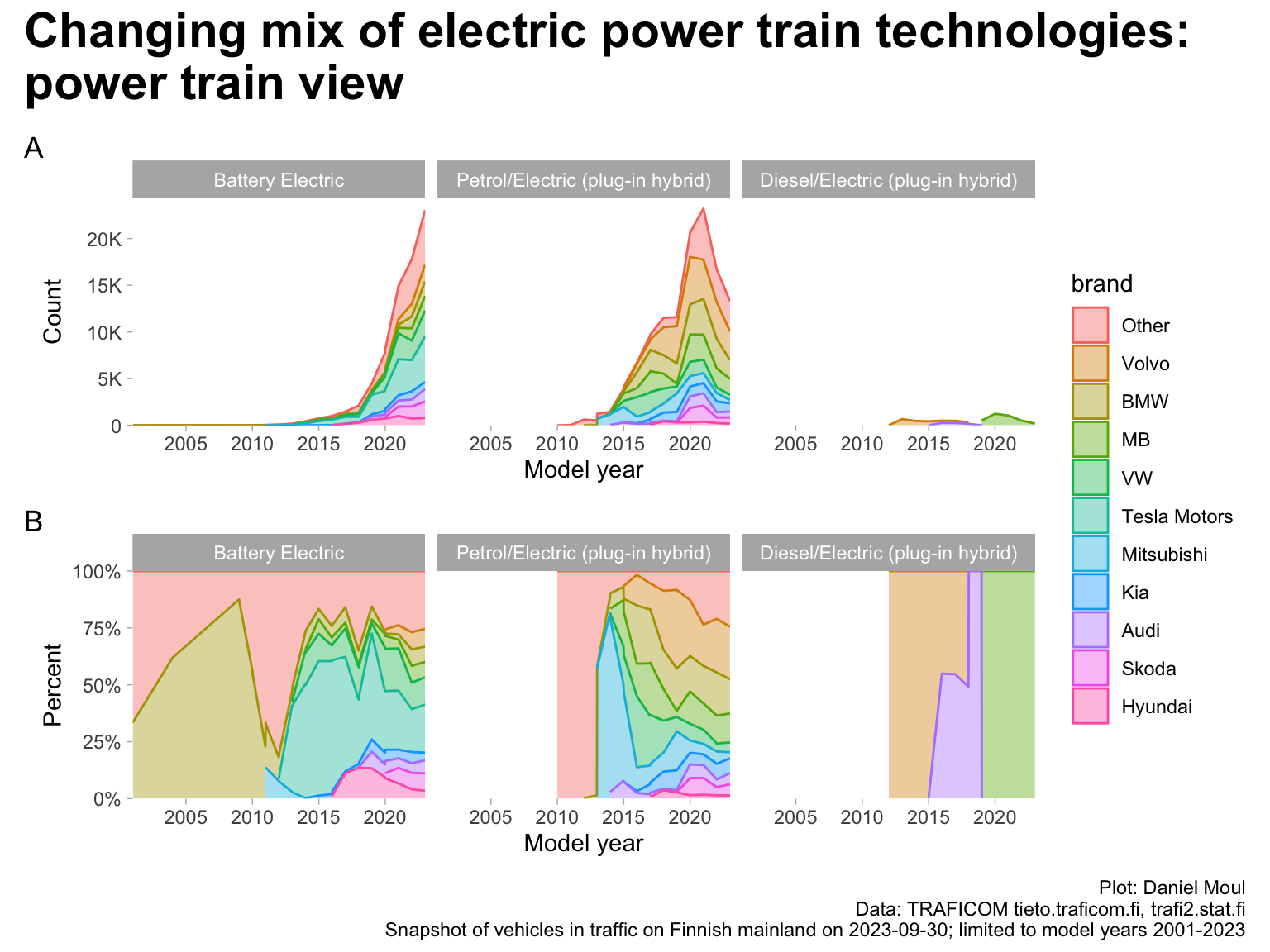
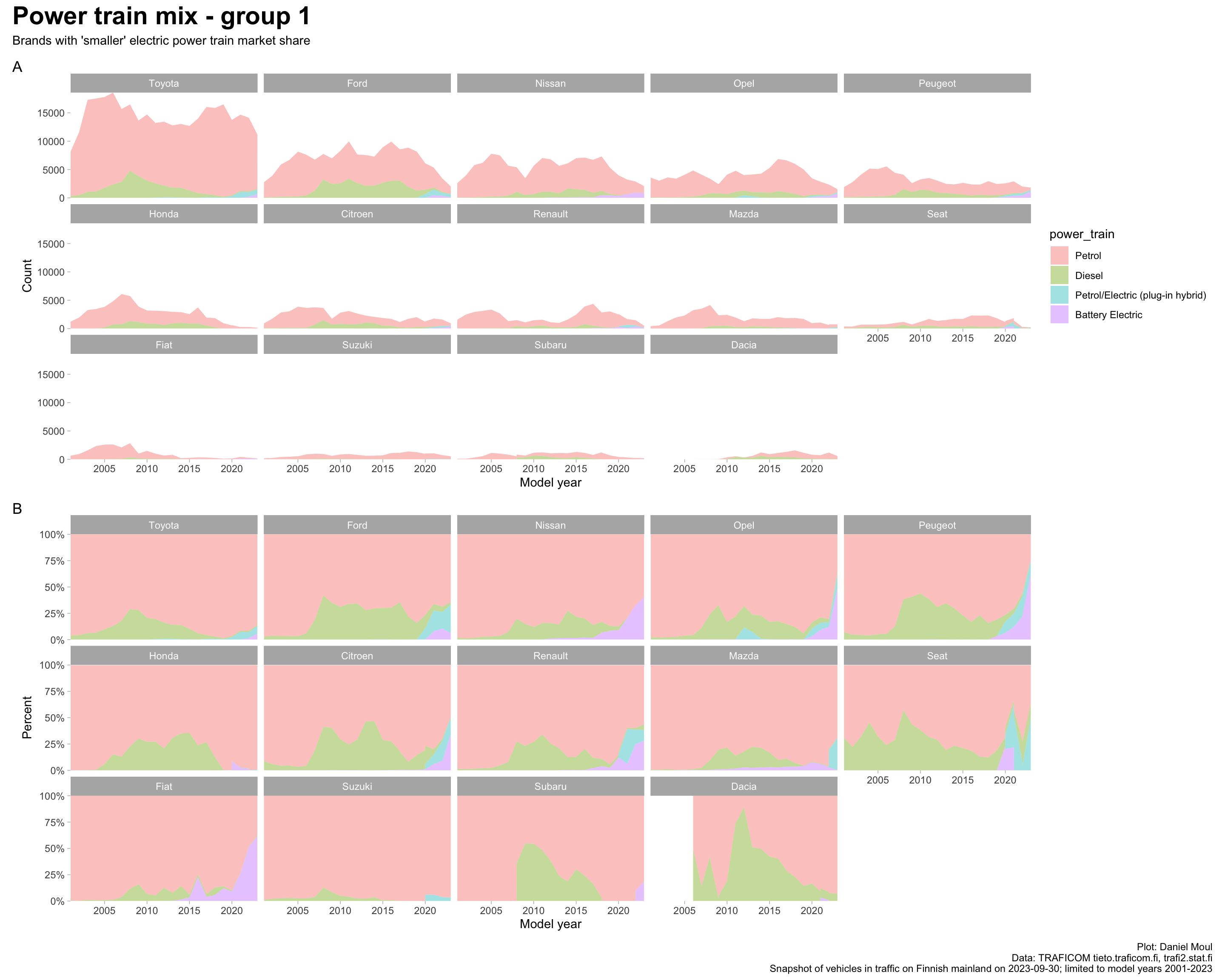
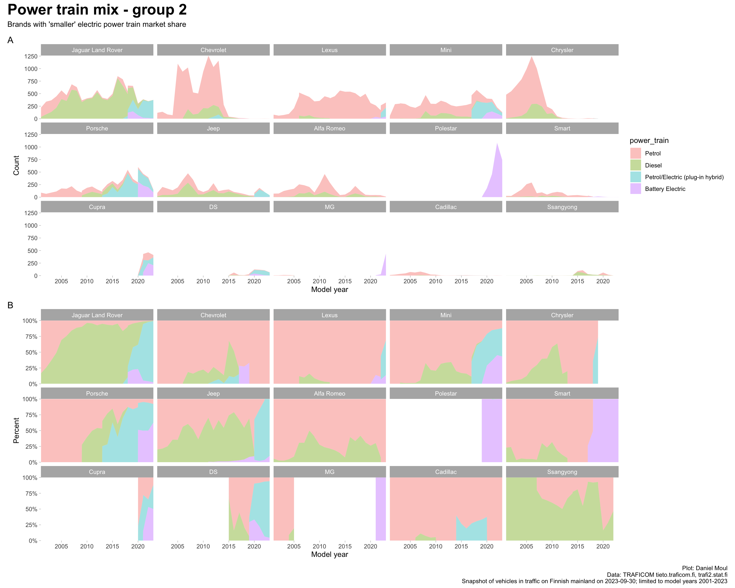
5.2.2 Looking only at brands with hybrid-electric and battery electric power trains

Diesel hybrid never really got going (Figure 5.8 panel A right facet), and while petrol hybrid gained significant share, it’s now in decline compared to battery electric. Tesla opened an early market share lead in battery electric market share.

Show the code

data_for_plot <- dta_by_brand_power_train |>
  filter(count > 0,
         str_detect(power_train, "Electric")) |>
  mutate(brand = fct_lump(brand, n = brand_cutoff_n, w = count)) |>
  summarize(count = sum(count),
          pct = sum(pct),
          .by = c(model_year, brand, power_train)) |>
  mutate(brand = fct_reorder(brand, -count, sum),
         power_train = fct_rev(power_train),
         power_train = fct_relevel(power_train, "Battery Electric"))

brands_electric_top <- data_for_plot |>
  distinct(brand) |>
  filter(brand != "Other") |>
  droplevels()

p1 <- data_for_plot |>
  ggplot() +
  geom_area(aes(model_year, count, color = brand, fill = brand, group = brand),
            show.legend = TRUE,
            alpha = 0.4) +
  scale_x_continuous(breaks = my_breaks_five_yearly$model_year,
                     expand = expansion(mult = c(0, 0))) +
  scale_y_continuous(labels = label_number(scale_cut = cut_short_scale()),
                     expand = expansion(mult = c(0, 0.05))) +
  facet_wrap( ~power_train) +
  labs(
    x = "Model year",
    y = "Count",
    tag = "A"
  )

p2 <- data_for_plot |>
  ggplot() +
  geom_area(aes(model_year, count, color = brand, fill = brand, group = brand),
            position = position_fill(),
            show.legend = FALSE,
            alpha = 0.4) +
  scale_x_continuous(breaks = my_breaks_five_yearly$model_year,
                     expand = expansion(mult = c(0, 0))) +
  scale_y_continuous(labels = label_percent(),
                     expand = expansion(mult = c(0, 0))) +
  facet_wrap( ~power_train) +
  labs(
    x = "Model year",
    y = "Percent",
    tag = "B"
  )

(p1 / p2) +
  plot_annotation(
    title = "Changing mix of electric power train technologies:\npower train view",
    caption = my_caption
  ) +
  plot_layout(guides = "collect")

Figure 5.8: Changing electric power train mix - power train view

Show the code

data_for_plot_tmp <- dta_by_brand_power_train |>
  filter(count > 0,
         str_detect(power_train, "Electric"))


brands_electric_top <- data_for_plot_tmp |>
  count(brand, wt = count, name = "count", sort = TRUE) |>
  head(10) |>
  select(brand)

data_for_plot <- data_for_plot_tmp |>
  inner_join(brands_electric_top,
             by = "brand") |>
  summarize(count = sum(count),
          pct = sum(pct),
          .by = c(model_year, brand, power_train)) |>
  mutate(brand = fct_lump(brand, brand_cutoff_n),
         brand = fct_reorder(brand, -count, sum),
         power_train = fct_relevel(power_train, "Battery Electric"),
         power_train = fct_rev(power_train)
         ) |>
  filter(brand != "Other") |>
  droplevels()

# brands_electric_top <- data_for_plot |>
#   distinct(brand) |>
#   filter(brand != "Other") |>
#   droplevels()

p1 <- data_for_plot |>
  ggplot() +
  geom_area(aes(model_year, count, fill = power_train, color = power_train),
           show.legend = FALSE,
           alpha = 0.4) +
  scale_x_continuous(breaks = my_breaks_five_yearly$model_year,
                     expand = expansion(mult = c(0, 0))) +
  scale_y_continuous(expand = expansion(mult = c(0, 0.05))) +
  facet_wrap( ~ brand) +
  labs(
    x = "Model year",
    y = "Count",
    tag = "A"
  )

p2 <- data_for_plot |>
  ggplot() +
  geom_area(aes(model_year, pct, fill = power_train, color = power_train),
           position = position_fill(),
           alpha = 0.4) +
  scale_x_continuous(breaks = my_breaks_five_yearly$model_year,
                     expand = expansion(mult = c(0, 0))) +
  scale_y_continuous(labels = label_percent(),
                     expand = expansion(mult = c(0, 0))) +
  facet_wrap( ~ brand) +
  labs(
    x = "Model year",
    y = "Percent",
    tag = "B"
  )

p1 + p2 +
  plot_annotation(
    title = "Changing mix of hybrid and electric power train technologies: brand view",
    subtitle = glue("Top brands with most hybrid + electric market share"),
    caption = my_caption
  ) +
  plot_layout(guides = "collect")

Figure 5.9: Changing hybrid and electric power train mix - brand view

5.2.3 Brands not in the top 10 electric power trains.

Show the code

dta_by_smaller_brand_electric_power_train <- dta_by_brand_power_train |>
  filter(count > 0) |>
  mutate(brand = as.character(brand)) |>
  anti_join(brands_electric_top |>
              mutate(brands_electric_top = as.character(brands_electric_top)),
            by = join_by(brand))

There are 61 brands that are not in the top 10 electric vehicle market share that have sold at least one electric or hybrid vehicle.

Show the code

data_for_plot <- dta_by_smaller_brand_electric_power_train |>
  filter(str_detect(power_train, "Petrol$|Diesel|Electric$|Electric.*plug")) |>
  droplevels() |>
  filter(any(str_detect(power_train, "Electric")),
         .by = brand) |>
  count(brand, power_train, wt = count) |>
  mutate(brand = fct_reorder(brand, n, sum),
         power_train = fct_reorder(power_train, n, sum)) |>
  arrange(brand, power_train)

brands_smaller_electric <- data_for_plot |>
  arrange(desc(n)) |>
  select(brand)

min_model_year_smaller_electric <- min(dta_by_smaller_brand_electric_power_train$model_year)
max_model_year_smaller_electric <- max(dta_by_smaller_brand_electric_power_train$model_year)

p1 <- data_for_plot |>
  ggplot() +
  geom_col(aes(n, brand, fill = power_train),
           show.legend = TRUE,
           alpha = 0.7) +
  scale_x_continuous(labels = label_number(scale_cut = cut_short_scale()),
                     expand = expansion(mult = c(0, 0.05))) +
  scale_fill_hue(direction = -1) +
  theme(legend.position = c(0.6, 0.3)) +
  labs(
    #subtitle = "All brands not in top 10",
    x = "Count",
    y = NULL,
    tag = "A"
  )

p2 <- data_for_plot |>
  filter(sum(n) < 5000,
         .by = brand) |>
  ggplot() +
  geom_col(aes(n, brand, fill = power_train),
           show.legend = FALSE,
           alpha = 0.7) +
  scale_fill_hue(direction = -1) +
  labs(
    subtitle = "Brands with less than 5000 vehicles (subset of A)",
    x = "Count",
    y = NULL,
    tag = "B"
  )

p1 + p2 +
  plot_annotation(
    title = "Brands with 'smaller' hybrid and electric power train market share",
    subtitle = "Vehicle count (four main power trains)",
    caption = my_caption
  )

Figure 5.10: Brands with ‘smaller’ hybrid and electric power train market share

Show the code

data_for_plot_tmp <- dta_by_smaller_brand_electric_power_train |>
  filter(power_train %in% c("Petrol",
                            "Diesel",
                            "Battery Electric",
                            "Petrol/Electric (plug-in hybrid)"
                            )) |>
  filter(any(str_detect(power_train, "Electric")),
         .by = brand) |>
  mutate(power_train = fct_rev(factor(power_train)),
         brand = fct_reorder(brand, -count, sum),
         ) |>
  arrange(brand)

define_brand_groupings <- data_for_plot_tmp |>
  distinct(brand) |>
  mutate(idx = row_number(),
         group_idx = floor(idx / 15) + 1
  )

data_for_plot_small_electric <- data_for_plot_tmp |>
  inner_join(define_brand_groupings, 
             by = join_by(brand))

Show the code

plot_brands_small_electric <- function(tbl, group_id) {
  
  # test
  # tbl = data_for_plot_small_electric
  # group_id = 2
  
  data_for_plot <- tbl |>
  filter(group_idx == group_id)
  
  p1 <- data_for_plot |>
    ggplot() +
    geom_area(aes(model_year, count, fill = power_train),
              show.legend = TRUE,
              alpha = 0.4) +
    scale_x_continuous(breaks = my_breaks_five_yearly$model_year,
                       expand = expansion(mult = c(0, 0))) +
    scale_y_continuous(expand = expansion(mult = c(0, 0))) +
    facet_wrap( ~ brand, ncol = 5) +
    labs(
      x = "Model year",
      y = "Count",
      tag = "A",
    )
  
  p2 <- data_for_plot |>
    ggplot() +
    geom_area(aes(model_year, count, fill = power_train),
              position = position_fill(),
              show.legend = FALSE,
              alpha = 0.4) +
    scale_x_continuous(breaks = my_breaks_five_yearly$model_year,
                       expand = expansion(mult = c(0, 0))) +
    scale_y_continuous(labels = label_percent(),
                       expand = expansion(mult = c(0, 0))) +
    facet_wrap( ~ brand, ncol = 5) +
    labs(
      x = "Model year",
      y = "Percent",
      tag = "B",
    )
  
  (p1 / p2) + 
    plot_annotation(
      title = glue("Power train mix - group {group_id}"),
      subtitle = "Brands with 'smaller' electric power train market share",
      caption = my_caption
    )
  
}

plot_brands_small_electric(data_for_plot_small_electric, group_id = 1)

Figure 5.11: Changing electric power train mix - brand view group 1

Show the code

plot_brands_small_electric(data_for_plot_small_electric, group_id = 2)

Figure 5.12: Changing electric power train mix - brand view group 2

Show the code

plot_brands_small_electric(data_for_plot_small_electric |>
                             mutate(brand = fct_relevel(brand, "Others", after = Inf)), 
                           group_id = 3)

Figure 5.13: Changing electric power train mix - brand view group 3

---

1. See also World Economic Forum and European Parliament FAQ 30-06-2023 20221019STO44572)