9  Consumer prices

Show the code
source(here::here("scripts/load-libraries.R"))

theme_set(theme_light() +
            theme(panel.grid.major = element_blank(),
                  panel.grid.minor = element_blank(),
                  plot.title = element_text(size = rel(2))))

my_caption_rbf = "Daniel Moul. Source: Reserve Bank of Fiji"
my_caption_fbos = "Daniel Moul. Source: Fiji Bureau of Statistics via Reserve Bank of Fiji"

The data used in this section comes from the Reserve Bank of Fiji and the US Federal Reserve Bank of Minneaopolis.

9.1 Consumer price index

The Reserve Bank of Fiji makes available historical consumer price data going back to 1991, rebased in 2005, 2008, 2011, and 2014. The CPI is based on the changing prices of a basket of representative products and services grouped in CPI component categories, and then the components are weighted to reflect consumer spending. The component categories changed between 2005 and 2008 (making comparisons between them difficult). Fortunately, only the weightings changed in subsequent rebases. Where year-to-year price changes were included in multiple rebases, I averaged them to calculate a single, simple, non-authoritative CPI for the entire period (Figure 9.1 panel B).
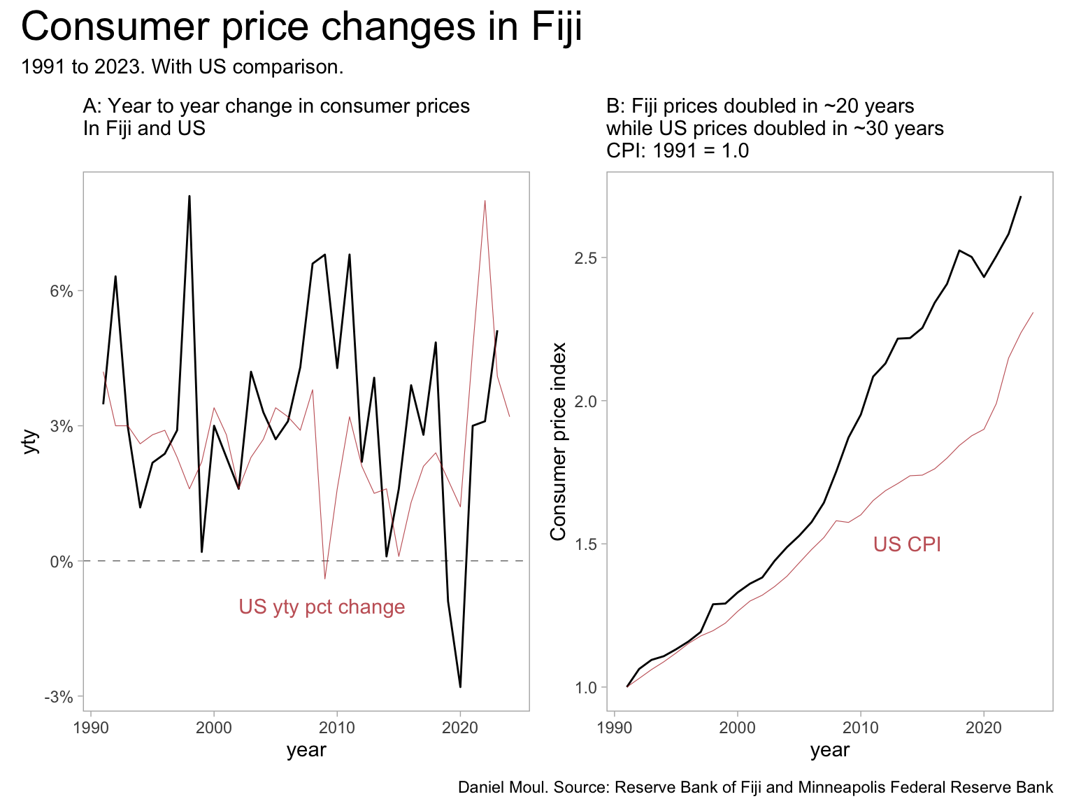
Show the code
cpi_2005_base_raw <- read_xlsx(here("data/raw/rbf/7.1-Consumer-Price-Index-fixed.xlsx"),
                   range = "A3:U28") |>
  clean_names() |>
  remove_empty(which = c("rows", "cols"))

cpi_2008_base_raw <- read_xlsx(here("data/raw/rbf/7.1-Consumer-Price-Index-fixed.xlsx"),
                   range = "A33:U40") |>
  clean_names() |>
  remove_empty(which = c("rows", "cols"))

cpi_2011_base_raw <- read_xlsx(here("data/raw/rbf/7.1-Consumer-Price-Index-fixed.xlsx"),
                   range = "A45:U55") |>
  clean_names() |>
  remove_empty(which = c("rows", "cols"))

cpi_2014_base_raw <- read_xlsx(here("data/raw/rbf/7.1-Consumer-Price-Index-fixed.xlsx"),
                   range = "A60:U70") |>
  clean_names() |>
  remove_empty(which = c("rows", "cols"))

cpi_merged <- bind_rows(
  cpi_2005_base_raw |>
    mutate(base = 2005),
  cpi_2008_base_raw |>
    mutate(base = 2008),
  cpi_2011_base_raw |>
    mutate(base = 2011),
  cpi_2014_base_raw |>
    mutate(base = 2014)
) |>
  rename(communications = communi_cations)

cpi_merged_long <- cpi_merged |>
  filter(base != 2005,
         period != "Weight") |>
  remove_empty(which = "cols") |>
  select(-year_on_year_percent_change, -all_items) |>
  relocate(base, .before = period) |>
  mutate(period = as.numeric(period),
         base = glue("base: {base}")) |> 
  pivot_longer(
    cols = clothing_footwear:recreation_culture,
    names_to = "metric",
    values_to = "value"
  ) |>
  mutate(metric = case_match(
    metric,
    "clothing_footwear"                          ~ "clothing_footwear",
    "transport"                                  ~ "transport",
    "food_and_non_alcoholic_beverage"            ~ "food_non_alcohol_bev",
    "alcoholic_beverages_tobacco_and_narcotics"  ~ "alcohol_tobacco_etc",
    "housing_water_elec_gas_and_other_fuels"     ~ "housing_water_elec_etc",
    "furnishings_hhld_equip_routine_hhld_maint"  ~ "furnishings_hhld_etc",
    "health"                                     ~ "health",
    "communications"                            ~ "communications",
    "recreation_culture"                         ~ "recreation_culture",
    .default = metric  # default just in case; shouldn't be needed
  ))

cpi_weights <- cpi_merged |>
  filter(base != 2005) |>
  remove_empty(which = "cols")

cpi <- cpi_merged |>
  select(period, year_on_year_percent_change, base) |>
  filter(period != "Weight") |>
  mutate(year = as.numeric(period)) |>
  summarize(yty = mean(year_on_year_percent_change) / 100,
            cpi = 0,
         .by = year) #|>
  # mutate(cpi = lag(cpi) * (1 + yty)) #lag(yty, default = 0)))

# since lag() doesn't seem to get the whole vector at the beginning of the call, I cannot 
# modify cpi while lagging it. So instead I use the following:
for(i in 1:length(cpi$yty)) {
   if(i == 1) {
    cpi$cpi[i] <- 1
  } else {
    cpi$cpi[i] <- cpi$cpi[i - 1] * (1 + cpi$yty[i])
  }
}

cpi_year_min <- min(cpi$year)
cpi_year_max <- max(cpi$year)

cpi_weights_tmp <- cpi_merged |>
  filter(base != 2005) |>
  remove_empty(which = "cols") |>
  relocate(base) |>
  select(-all_items) |>
  pivot_longer(
    cols = clothing_footwear:recreation_culture,
    names_to = "metric",
    values_to = "weight"
  ) |>
  mutate(metric = case_match(
    metric,
    "clothing_footwear"                          ~ "clothing_footwear",
    "transport"                                  ~ "transport",
    "food_and_non_alcoholic_beverage"            ~ "food_non_alcohol_bev",
    "alcoholic_beverages_tobacco_and_narcotics"  ~ "alcohol_tobacco_etc",
    "housing_water_elec_gas_and_other_fuels"     ~ "housing_water_elec_etc",
    "furnishings_hhld_equip_routine_hhld_maint"  ~ "furnishings_hhld_etc",
    "health"                                     ~ "health",
    "communications"                            ~ "communications",
    "recreation_culture"                         ~ "recreation_culture"
  ))
  
cpi_weights <- cpi_weights_tmp |>
  filter(base != 2005,
         period == "Weight") |>
  remove_empty(which = "cols") |>
  relocate(base) |>
  select(-period)

dta_for_cpi_weight_plot <- cpi_weights_tmp |>
  filter(base != 2005,
         period != "Weight") |>
  remove_empty(which = "cols") |>
  relocate(base) |>
  rename(value = weight) |>
  left_join(
    cpi_weights,
    by = c("base", "metric")
  )

us_cpi <- read_xlsx(here("data/raw/us-frb/us-cpi-historical.xlsx"),
                   skip = 7) |>
  clean_names() |>
  mutate(cpi_base_1991 = cpi / cpi[year == 1991])


Show the code
p1 <- cpi |>
  ggplot(aes(year, yty)) +
  geom_hline(yintercept = 0, lty = 2, linewidth = 0.15, alpa = 0.5) +
  geom_line() +
  geom_line(data = us_cpi |>
              filter(year >= 1991),
            aes(year, annual_pct_change),
            color = "firebrick", linewidth = 0.2,
            alpha = 0.75) +
  annotate("text", x = 2002, y = -0.01, label = "US yty pct change",
           hjust = 0, color = "firebrick", alpha = 0.75) +
  scale_y_continuous(labels = label_percent()) +
  labs(
    subtitle = glue("A: Year to year change in consumer prices",
                    "\nIn Fiji and US")
  )

p2 <- cpi |>
  ggplot() +
  geom_line(aes(year, cpi)) +
  geom_line(data = us_cpi |>
              filter(year >= 1991),
            aes(year, cpi_base_1991),
            color = "firebrick", linewidth = 0.2,
            alpha = 0.75) +
  annotate("text", x = 2011, y = 1.5, label = "US CPI",
           hjust = 0, color = "firebrick", alpha = 0.75) +
  labs(
    subtitle = glue("B: Fiji prices doubled in ~20 years",
                    "\nwhile US prices doubled in ~30 years",
                    "\nCPI: {cpi_year_min} = 1.0"),
    y = "Consumer price index"
  )

p1 + p2 +
  plot_annotation(
    title = "Consumer price changes in Fiji",
    subtitle = glue("{cpi_year_min} to {cpi_year_max}. With US comparison."),
    caption = paste0(my_caption_rbf,
                     " and Minneapolis Federal Reserve Bank")
  )
Figure 9.1: Fiji consumer price index


9.2 Impact on consumers

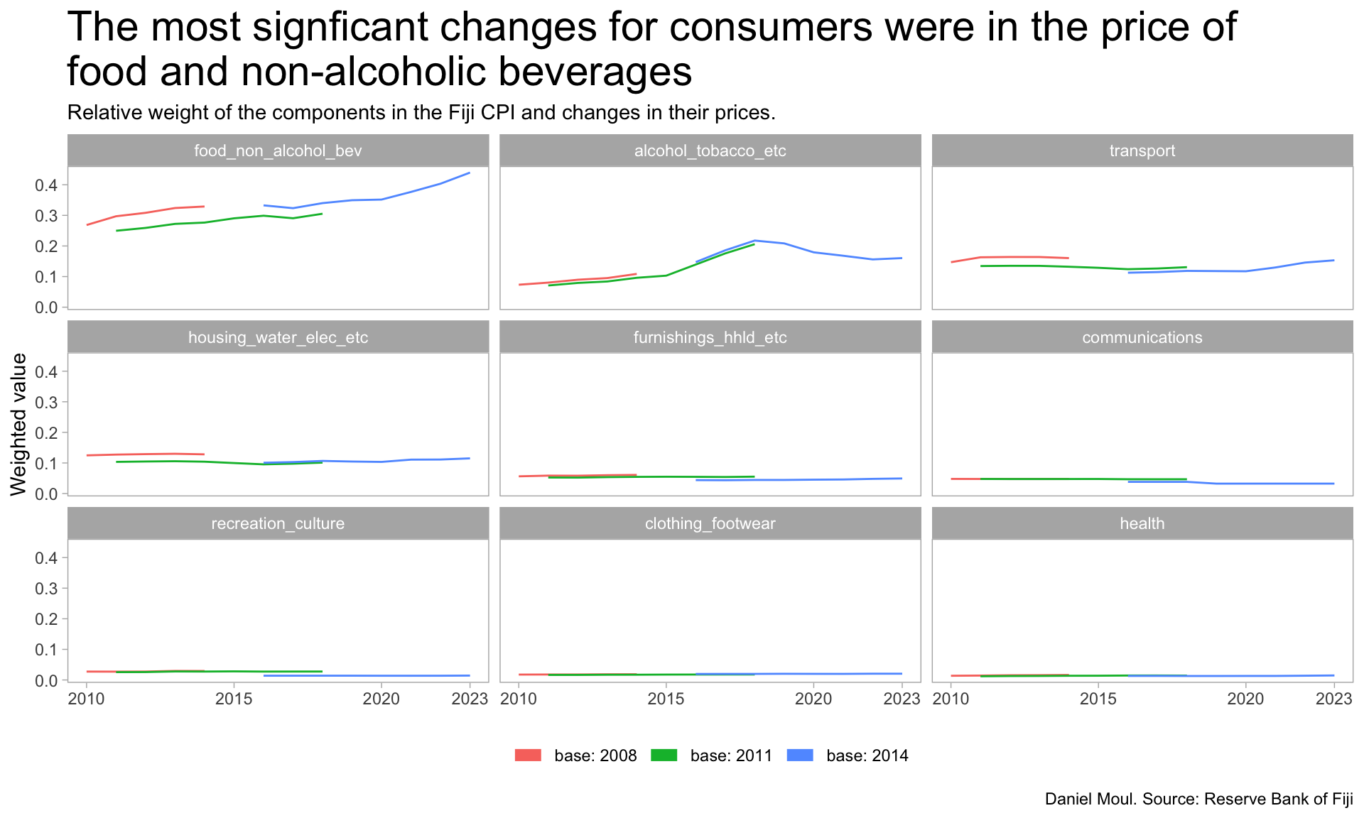
“Food and non-alcoholic beverages” is heaviest weighted component of the CPI, and price increases in this component since the COVID-19 pandemic have been especially painful. While I was in Fiji friends and relatives were talking about the current “affordability crisis”.

In Figure 9.2 and Figure 9.3 \[component\ weighted\ value = component\ weight * relative \ price\] and scaled such that the \[\sum{component\ weighted\ values} = 1.0,\ for\ all\ component\ weighted\ values\ in\ 2023\]


Show the code
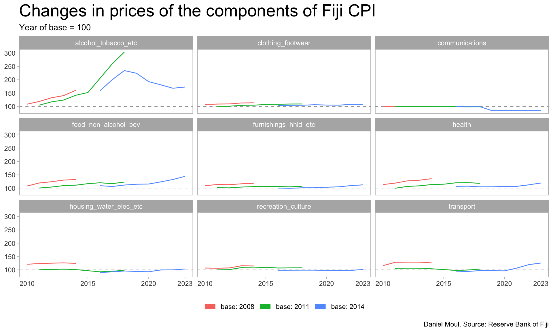
dta_for_plot <- dta_for_cpi_weight_plot |>
  mutate(base = glue("base: {base}"),
         period = as.numeric(period),
         weighted_value = weight * value,
         metric = fct_reorder(metric, -weighted_value, min),
         weighted_value_scaled = weighted_value / sum(weighted_value[period == 2023])
         )

dta_for_plot |>
  ggplot(aes(period, weighted_value_scaled, color = base, group = base)) +
  geom_line() +
  scale_x_continuous(breaks = c(2010, 2015, 2020, 2023)) +
  facet_wrap(~metric) +
  guides(color = guide_legend(ncol = 3,
                              override.aes = list(linewidth = 3))
         ) +
  theme(legend.position = "bottom") +
  labs(
    title = glue("The most signficant changes for consumers were in the price of", 
                 "\nfood and non-alcoholic beverages"),
    subtitle = glue("Relative weight of the components in the Fiji CPI and changes in their prices."),
    x = NULL,
    y = "Weighted value",
    color = NULL,
    caption = my_caption_rbf
  )
Figure 9.2: Fiji consumer price index component changes with weightings


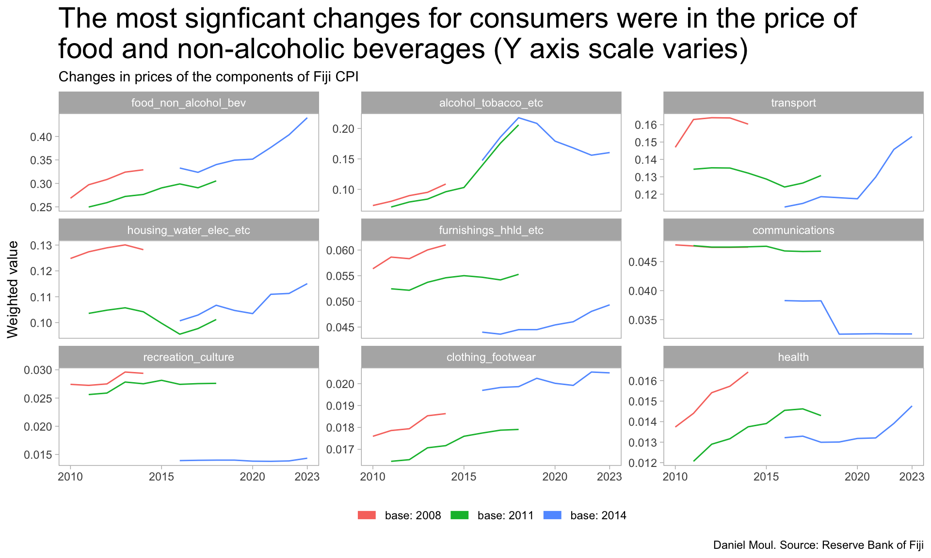
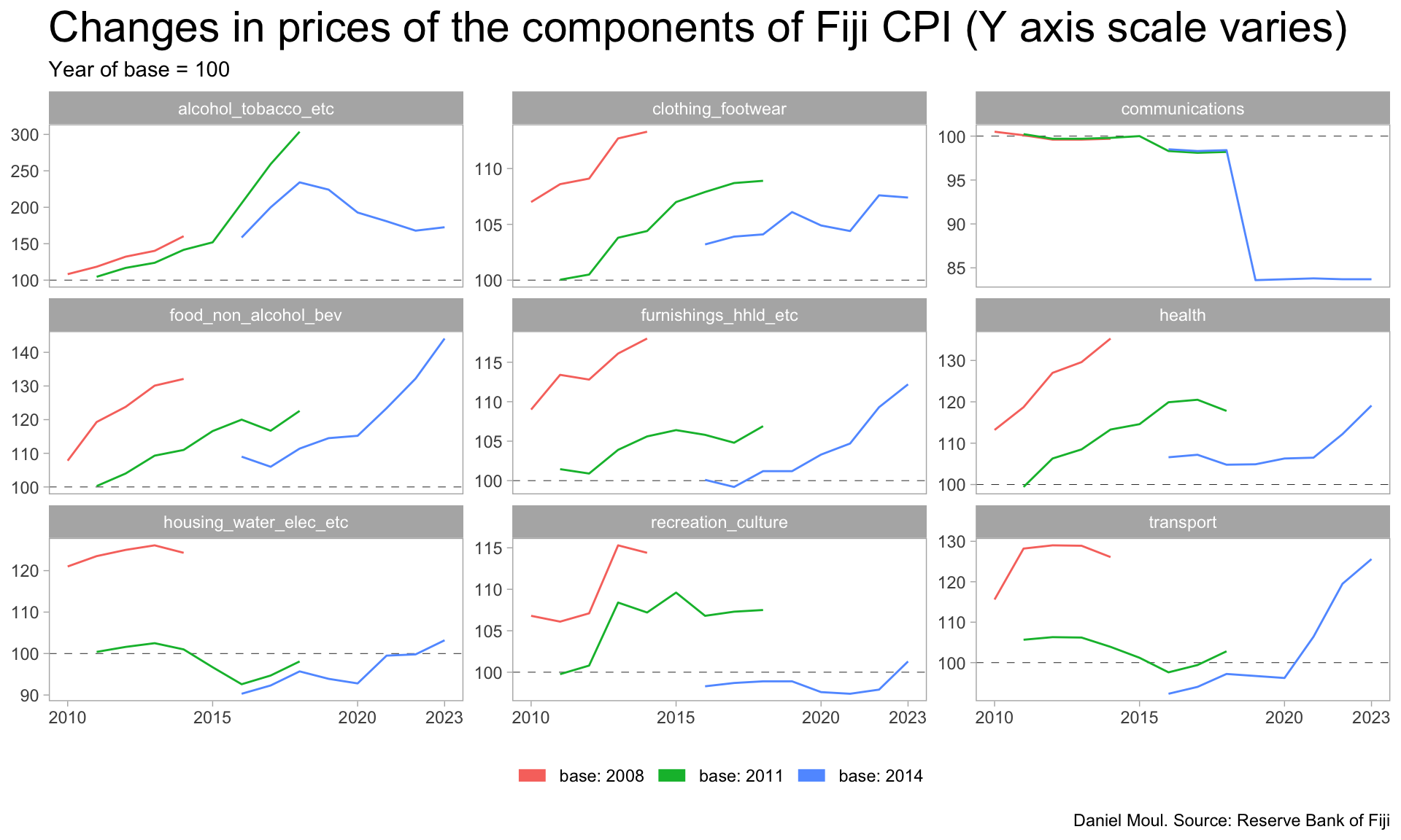
Figure 9.3 presents the same data with varying Y axes, which makes the trends within components more visible.

Show the code
dta_for_plot |>
  ggplot(aes(period, weighted_value_scaled, color = base, group = base)) +
  geom_line() +
  scale_x_continuous(breaks = c(2010, 2015, 2020, 2023)) +
  facet_wrap(~metric, scales = "free_y") +
  guides(color = guide_legend(ncol = 3,
                              override.aes = list(linewidth = 3))
         ) +
  theme(legend.position = "bottom") +
  labs(
    title = glue("The most signficant changes for consumers were in the price of", 
                 "\nfood and non-alcoholic beverages (Y axis scale varies)"),
    subtitle = glue("Changes in prices of the components of Fiji CPI"),
    x = NULL,
    y = "Weighted value",
    color = NULL,
    caption = my_caption_rbf
  )
Figure 9.3: Fiji consumer price index component changes with weightings (Y axis scale varies)


9.3 CPI components and rebases

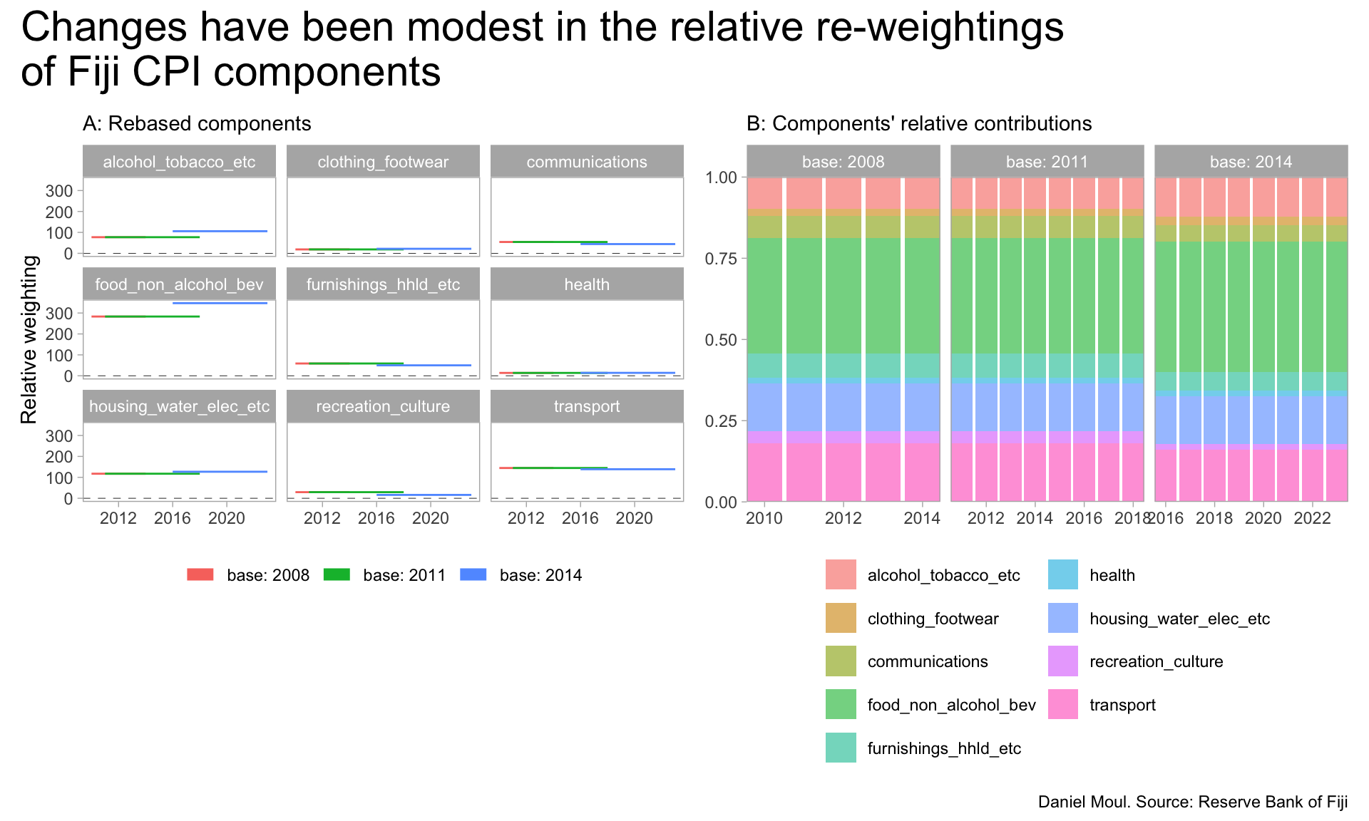
The components and their weightings reflect the Reserve Bank’s understanding of how people in Fiji spend their money. In each rebase, the reweightings were scaled to sum to 1000 (Figure 9.4 panel A).

Show the code
p1 <- dta_for_cpi_weight_plot |>
  mutate(base = glue("base: {base}"),
         period = as.numeric(period)) |>
  ggplot(aes(period, weight, color = base, group = base)) +
  geom_hline(yintercept = 0, lty = 2, linewidth = 0.15, alpa = 0.5) +
  geom_line() +
  guides(color = guide_legend(override.aes = list(linewidth = 3))) +
  facet_wrap(~metric) +
  theme(legend.position = "bottom") +
  labs(
    subtitle = "A: Rebased components",
    x = NULL,
    y = "Relative weighting",
    color = NULL
    )

p2 <- dta_for_cpi_weight_plot |>
  mutate(base = glue("base: {base}"),
         period = as.numeric(period)) |>
  ggplot(aes(period, weight, fill = metric)) +
  geom_col(position = position_fill(),
           alpha = 0.6,
           na.rm = TRUE) +
  scale_x_continuous(expand = expansion(mult = c(0,0)),
                   breaks = 2010 + 2 * 0:10) +
  scale_y_continuous(expand = expansion(mult = c(0,0))) +
  theme(legend.position = "bottom") +
  facet_wrap(~base, scales ="free_x") +
  labs(
    subtitle = "B: Components' relative contributions",
    x = NULL,
    y = NULL,
    fill = NULL
  )

p1 + p2 +
  plot_annotation(
    title = glue("Changes have been modest in the relative re-weightings",
                 "\nof Fiji CPI components"),
    caption = my_caption_rbf
  ) +
  guides(fill = guide_legend(ncol = 2))
Figure 9.4: Fiji consumer price index weightings


Ignoring component weightings, Figure 9.5 and Figure 9.6 present the degree of inflation within each component.

Show the code
cpi_merged_long |>
  ggplot(aes(period, value, color = base, group = base)) +
  geom_hline(yintercept = 100, lty = 2, linewidth = 0.15, alpa = 0.5) +
  geom_line() +
  scale_x_continuous(breaks = c(2010, 2015, 2020, 2023)) +
  facet_wrap(~metric) +
  guides(color = guide_legend(ncol = 3,
                              override.aes = list(linewidth = 3))
         ) +
  theme(legend.position = "bottom") +
  labs(
    title = "Changes in prices of the components of Fiji CPI",
    subtitle = "Year of base = 100",
    x = NULL,
    y = NULL,
    color = NULL,
    caption = my_caption_rbf
  )
Figure 9.5: Fiji consumer price index component price changes


Figure 9.6 presents the same data with varying Y axes, which makes the trends within components more visible.

Show the code
cpi_merged_long |>
  ggplot(aes(period, value, color = base, group = base)) +
  geom_hline(yintercept = 100, lty = 2, linewidth = 0.15, alpa = 0.5) +
  geom_line() +
  scale_x_continuous(breaks = c(2010, 2015, 2020, 2023)) +
  facet_wrap(~metric, scales = "free_y") +
  guides(color = guide_legend(ncol = 3,
                              override.aes = list(linewidth = 3))
         ) +
  theme(legend.position = "bottom") +
  labs(
    title = "Changes in prices of the components of Fiji CPI (Y axis scale varies)",
    subtitle = "Year of base = 100",
    x = NULL,
    y = NULL,
    color = NULL,
    caption = my_caption_rbf
  )
Figure 9.6: Fiji consumer price index component price changes (Y axis scale varies)


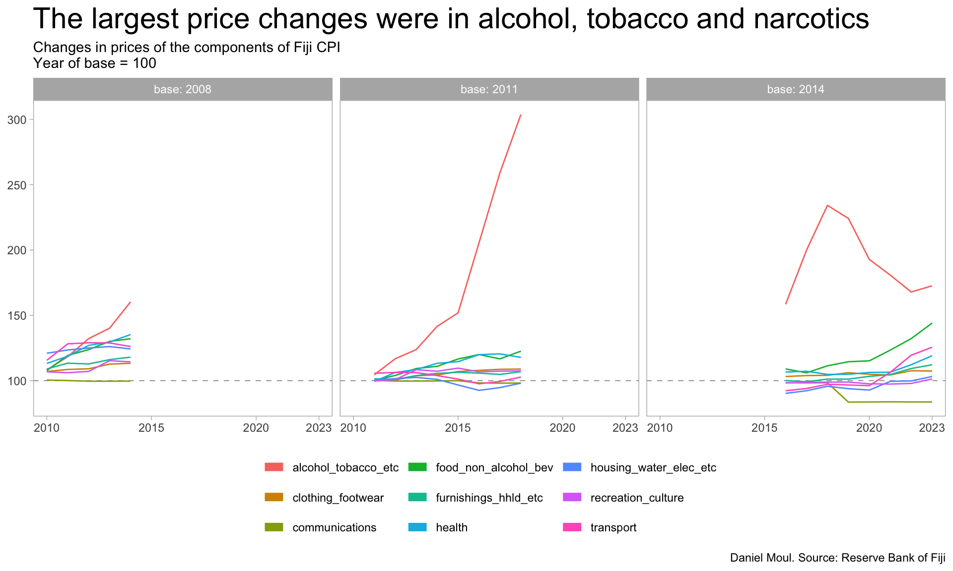
Plotting all components for each rebase (Figure 9.7) makes visible the wide swings in relative prices in the ‘alcohol, tobacco and narcotics’ component.

Show the code
cpi_merged_long |>
  ggplot(aes(period, value, color = metric, group = metric)) +
  geom_hline(yintercept = 100, lty = 2, linewidth = 0.15, alpa = 0.5) +
  geom_line() +
  scale_x_continuous(breaks = c(2010, 2015, 2020, 2023)) +
  facet_wrap(~base) +
  guides(color = guide_legend(ncol = 3,
                              override.aes = list(linewidth = 3))
         ) +
  theme(legend.position = "bottom") +
  labs(
    title = "The largest price changes were in alcohol, tobacco and narcotics",
    subtitle = glue("Changes in prices of the components of Fiji CPI",
                    "\nYear of base = 100"),
    x = NULL,
    y = NULL,
    color = NULL,
    caption = my_caption_rbf
  )
Figure 9.7: Fiji consumer price index component price changes plotted together. Largest increases and swings in prices were in the ‘alcohol, tobacco and narcotics’ component