7  Overseas arrivals, tourism revenue, and hotel nights

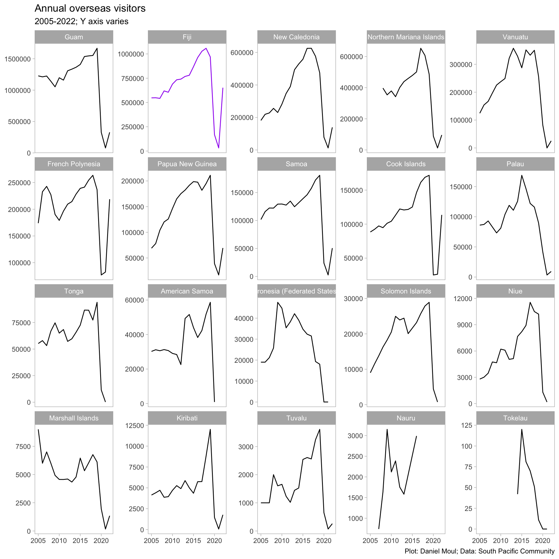
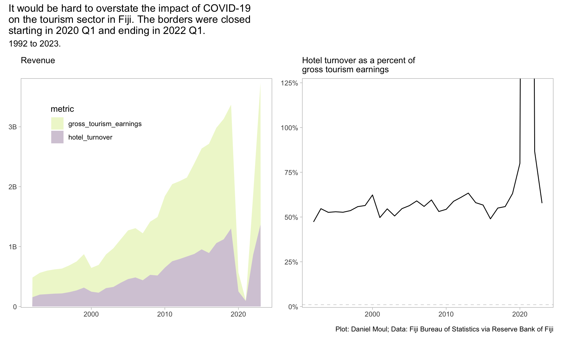
Among the PICTs, tourism is a significant source of foreign currency and local employment. The COVID-19 pandemic shut down most overseas travel, and as of 2022 annual numbers did not returned to pre-pandemic trends. Overseas visitors include sea and air arrivals. It includes excursionists/same-day-visitors i.e. visitors from cruise ships.

Fiji is second, behind only Guam in number of overseas arrivals. Are U.S. active military personnel included in Guam’s numbers? If so then Fiji would be first in yearly non-military visitors: mainly people traveling for holiday, work, or visiting friends and family.

7.1 Overseas visitors

Show the code
source(here::here("scripts/load-libraries.R"))

theme_set(theme_light() +
            theme(panel.grid.major = element_blank(),
                  panel.grid.minor = element_blank()))

options(scipen = 5)

my_caption <- "Plot: Daniel Moul; Data: South Pacific Community"
my_caption_fbos <- "Plot: Daniel Moul; Data: Fiji Bureau of Statistics via Reserve Bank of Fiji"
Show the code
visitors_all_cat <- read_csv(here("./data/raw/overseas-visitor-arrivals/SPC-DF_OVERSEAS_VISITORS-2.0-all.csv"),
               show_col_types = FALSE) |>
  clean_names() |>
  remove_empty(which = "cols")

visitors_total <- visitors_all_cat |>
  filter(overseas_visitors_type_2 == "Total") |>
  mutate(place = fct_reorder(pacific_island_countries_and_territories, -obs_value, sum)) |>
  mutate(max_annual = max(obs_value),
         pct_of_max = obs_value / max_annual,
         min_year = min(time_period),
         max_year = max(time_period),
         pct_of_first_year = obs_value / obs_value[time_period == min_year],
         .by = pacific_island_countries_and_territories)
Show the code
fname <- here("./data/raw/rbf/5.4-Visitors-Arrivals-Number-by-Country-of-Residence.xlsx")
visitors_by_country_raw <- readxl::read_xlsx(fname,
                                             sheet = "Table 44",
                                             range = "A2:K43") |>
  clean_names() |>
  remove_empty(which = "cols") |>
  rename(nz = new_zealand,
         usa = "united_states_of_america",
         uk = "united_kingdom",
         europe = "continental_europe") |>
  select(-total)

# mutate(m = mean(c_across(x:z)))

visitors_by_country_long <- visitors_by_country_raw |>
  rowwise() |>
  mutate(total = sum(c_across(australia:others))) |>
  pivot_longer(cols = australia:total,
               names_to = "country",
               values_to = "visitors") |>
  mutate(country = fct_reorder(country, -visitors, sum)) |>
  mutate(pct_of_yearly = visitors / sum(visitors),
         .by = period) |>
  mutate(visitors_normalized = visitors / visitors[period == 1983],
         yty_growth = visitors / lag(visitors, default = NA) - 1,
         .by = country)

# https://en.wikipedia.org/wiki/Fiji_coup
# Also including the 2009 constitutional crisis
# https://en.wikipedia.org/wiki/2009_Fijian_constitutional_crisis
coup_years <- tibble(
  period = c(1987, 2000, 2006, 2009)
)

Most PICTs experienced a positive trend in annual visitors until the COVID-19 pandemic.

Show the code
visitors_total |>
  mutate(place = fct_reorder(pacific_island_countries_and_territories, -obs_value, sum)) |>
  ggplot() +
  geom_line(aes(time_period, obs_value, 
                color = if_else(place == "Fiji",
                                     "purple", 
                                     "black"))) +
  
  scale_color_identity() +
  facet_wrap(~place, scales = "free_y") +
  labs(
    title = "Annual overseas visitors",
    subtitle = "2005-2022; Y axis varies",
    x = NULL,
    y = NULL,
    caption = my_caption
  )
Figure 7.1: Annual overseas visitors


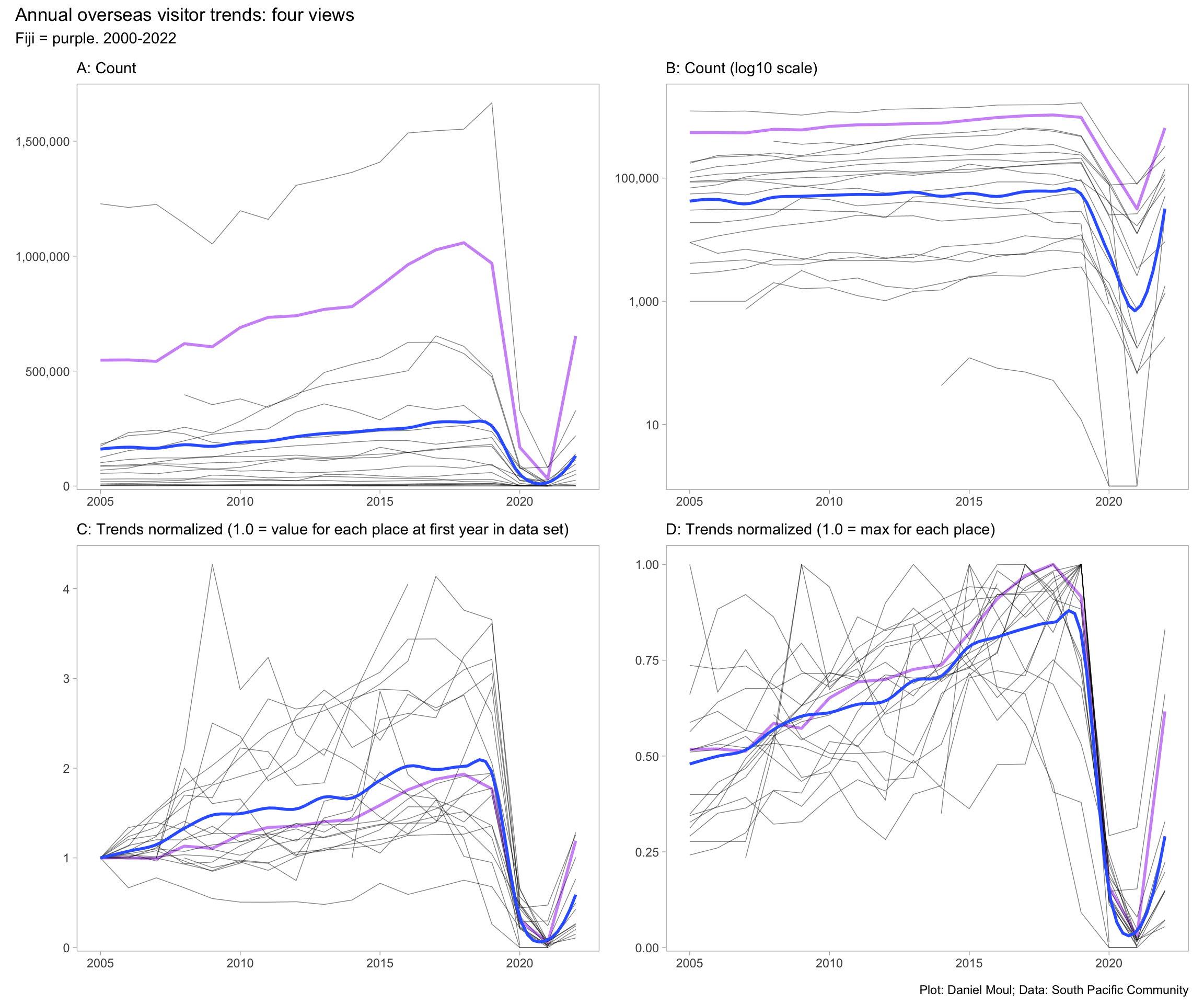
There are many ways one could compare the overseas visitors numbers among PICTs. I offer four below.

Show the code
p0 <- visitors_total |>
  mutate(place = fct_reorder(pacific_island_countries_and_territories, -obs_value, sum)) |>
  ggplot() +
  geom_line(aes(time_period, obs_value + 1, 
                color = if_else(place == "Fiji",
                                     "purple", 
                                     "black"),
                linewidth = if_else(place == "Fiji",
                                     1, 
                                     0),
                group = place),
            alpha = 0.5
            ) +
  geom_smooth(aes(time_period, obs_value + 1),
              method = "loess", formula = 'y ~ x',
              span = 0.2, se = FALSE) +
  scale_color_identity() +
  scale_linewidth_continuous(range = c(0.25, 1.0)) +
  scale_y_continuous(expand = expansion(mult = c(0.01, 0.05)),
                     labels = label_number(big.mark = ",")) +
  guides(linewidth = "none") +
  labs(
    subtitle = "A: Count",
    x = NULL,
    y = NULL
  )

p1 <- visitors_total |>
  mutate(place = fct_reorder(pacific_island_countries_and_territories, -obs_value, sum)) |>
  ggplot() +
  geom_line(aes(time_period, obs_value + 1, 
                color = if_else(place == "Fiji",
                                     "purple", 
                                     "black"),
                linewidth = if_else(place == "Fiji",
                                     1, 
                                     0),
                group = place),
            alpha = 0.5
            ) +
  geom_smooth(aes(time_period, obs_value + 1),
              method = "loess", formula = 'y ~ x',
              span = 0.2, se = FALSE) +
  scale_color_identity() +
  scale_linewidth_continuous(range = c(0.25, 1.0)) +
  scale_y_log10(expand = expansion(mult = c(0.01, 0.05)),
                labels = label_number(big.mark = ",")) +
  guides(linewidth = "none") +
  labs(
    subtitle = "B: Count (log10 scale)",
    x = NULL,
    y = NULL
  )

p2 <- visitors_total |>
  mutate(place = fct_reorder(pacific_island_countries_and_territories, -obs_value, sum)) |>
  ggplot() +
  geom_line(aes(time_period, pct_of_first_year, 
                color = if_else(place == "Fiji",
                                     "purple", 
                                     "black"),
                linewidth = if_else(place == "Fiji",
                                     1, 
                                     0),
                group = place),
            alpha = 0.5
            ) +
  geom_smooth(aes(time_period, pct_of_first_year),
              method = "loess", formula = 'y ~ x',
              span = 0.2, se = FALSE) +
  scale_color_identity() +
  scale_linewidth_continuous(range = c(0.25, 1.0)) +
  scale_y_continuous(expand = expansion(mult = c(0.01, 0.05)),
                     labels = label_number(big.mark = ",")) +
  guides(linewidth = "none") +
  labs(
    subtitle = "C: Trends normalized (1.0 = value for each place at first year in data set)",
    x = NULL,
    y = NULL
  )

p3 <- visitors_total |>
  mutate(place = fct_reorder(pacific_island_countries_and_territories, -obs_value, sum)) |>
  ggplot() +
  geom_line(aes(time_period, pct_of_max, 
                color = if_else(place == "Fiji",
                                     "purple", 
                                     "black"),
                linewidth = if_else(place == "Fiji",
                                     1, 
                                     0),
                group = place),
            alpha = 0.5
            ) +
  geom_smooth(aes(time_period, pct_of_max),
              method = "loess", formula = 'y ~ x',
              span = 0.2, se = FALSE) +
  scale_color_identity() +
  scale_linewidth_continuous(range = c(0.25, 1.0)) +
  scale_y_continuous(expand = expansion(mult = c(0.01, 0.05)),
                     labels = label_number(big.mark = ",")) +
  guides(linewidth = "none") +
  labs(
    subtitle = "D: Trends normalized (1.0 = max for each place)",
    x = NULL,
    y = NULL
  )

p0 + p1 + p2 + p3 +
  plot_annotation(
    title = "Annual overseas visitor trends: four views",
    subtitle = "Fiji = purple. 2000-2022",
    caption = my_caption
  )
Figure 7.2: Annual overseas visitor trends: four views


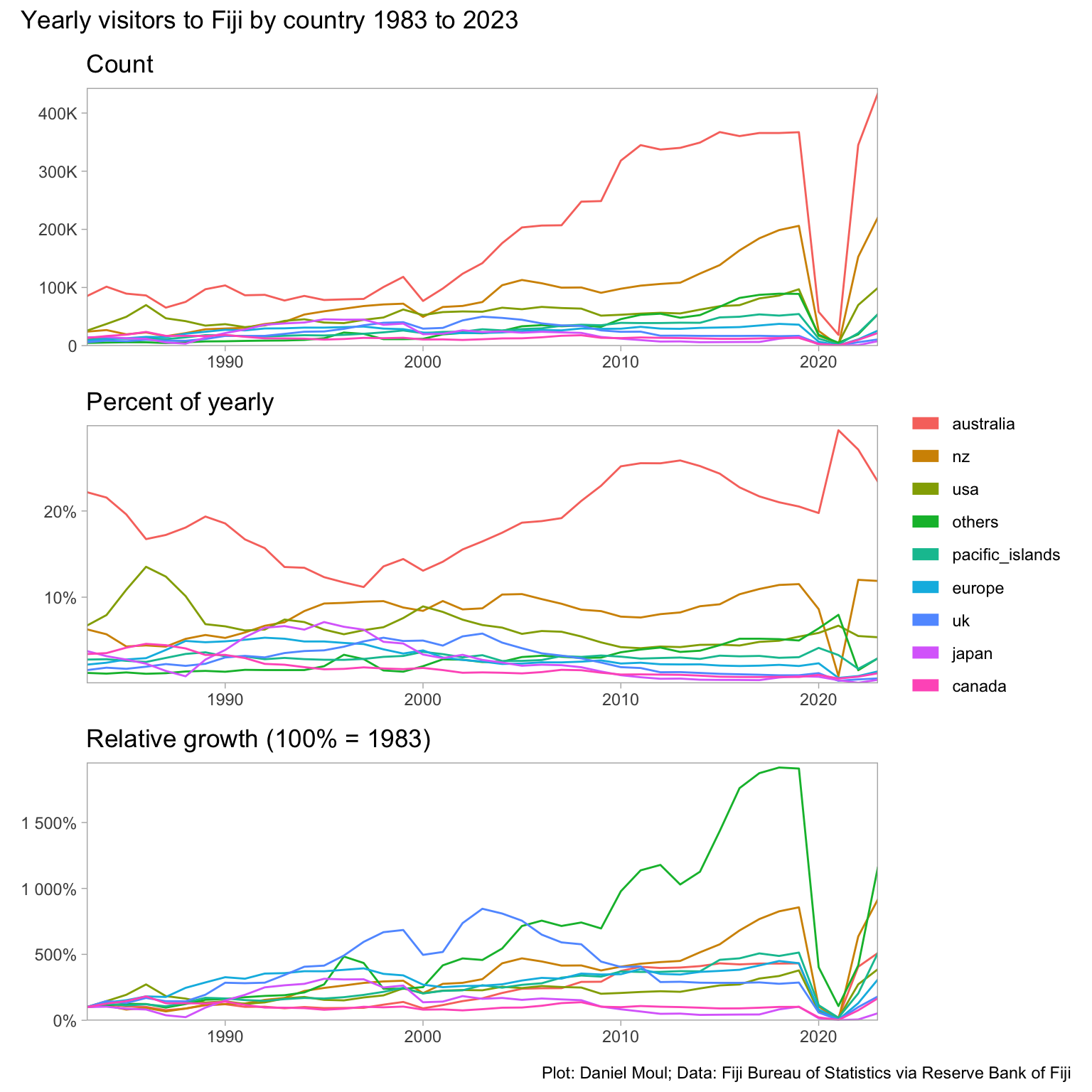
7.2 Visitors by country

Show the code
dta_for_plot <- visitors_by_country_long |>
  filter(country != "total")

year_min <- min(dta_for_plot$period)
year_max <- max(dta_for_plot$period)

p1 <- dta_for_plot |>
  ggplot() +
  geom_line(aes(x = period, y = visitors, color = country),
            show.legend = FALSE) +
  scale_x_continuous(expand = expansion(mult = c(0, 0))) +
  scale_y_continuous(expand = expansion(mult = c(0.002, 0.02)),
                     labels = label_number(scale_cut = cut_short_scale())) +
  labs(
    title = glue("Count"),
    x = NULL,
    y = NULL
  )

p2 <- dta_for_plot |>
  ggplot() +
  geom_line(aes(x = period, y = pct_of_yearly, color = country),
            show.legend = FALSE) +
  scale_x_continuous(expand = expansion(mult = c(0, 0))) +
  scale_y_continuous(expand = expansion(mult = c(0.002, 0.02)),
                     labels = label_percent()) +
  guides(color = guide_legend(override.aes = list(linewidth = 3))) +
  labs(
    title = glue("Percent of yearly"),
    x = NULL,
    y = NULL,
    color = NULL
  )

p3 <- dta_for_plot |>
  ggplot() +
  geom_line(aes(x = period, y = visitors_normalized, color = country),
            show.legend = TRUE) +
  scale_x_continuous(expand = expansion(mult = c(0, 0))) +
  scale_y_continuous(expand = expansion(mult = c(0.002, 0.02)),
                     labels = label_percent()) +
  guides(color = guide_legend(override.aes = list(linewidth = 3))) +
  labs(
    title = glue("Relative growth (100% = 1983)"),
    x = NULL,
    y = NULL,
    color = NULL
  )

p1 / p2 / p3 +
  plot_annotation(
    title = glue("Yearly visitors to Fiji by country {year_min} to {year_max}"),
    # subtitle = "Vertical lines are years with coups or constitutional crises",
    caption = my_caption_fbos
  ) +
  plot_layout(guides = "collect")
Figure 7.3: Annual overseas visitor by country


Show the code
dta_for_plot <- visitors_by_country_long |>
  filter(country != "total",
         period < 2020)

year_min <- min(dta_for_plot$period)
year_max <- max(dta_for_plot$period)

dta_for_plot |>
  ggplot(aes(x = period, y = yty_growth, color = country)) +
  geom_vline(xintercept = coup_years$period, lty = 2, linewidth = 0.25, alpha = 0.4) +
  geom_hline(yintercept = 0, linewidth = 0.25, alpha = 0.4) +
  geom_point(size = 1.0, alpha = 0.4,
             na.rm = TRUE) +
  geom_smooth(method = 'loess', formula = 'y ~ x', se = TRUE,
              linewidth = 0.75,
              fill = "grey", alpha = 0.25,
              na.rm = TRUE) +
  scale_x_continuous(expand = expansion(mult = c(0.01, 0.01))) +
  scale_y_continuous(expand = expansion(mult = c(0.002, 0.02)),
                     labels = label_percent()) +
  guides(color = "none") +
  coord_cartesian(ylim = c(NA, 0.55)) +
  facet_wrap(~country) +
  labs(
    title = glue("Year-to-year growth in visitors to Fiji by country {year_min} to {year_max}"),
    subtitle = glue("Vertical lines are years with political instability*",
                    "\nNot surprising that those years saw significant drops in visitors", 
                    " compared to the year prior"),
    x = NULL,
    y = NULL,
    color = NULL,
    caption = glue(my_caption_fbos,
                   "\n*Coup or constitutional crisis",
                   "\nNot showing one Japanese outlier > 50%")
  )
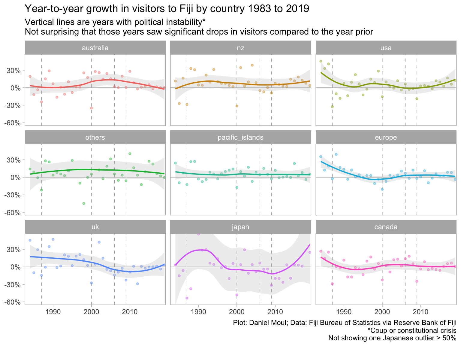
Figure 7.4: Year-to-year growth rate in overseas visitors by country


Show the code
visitors_for_table <- visitors_by_country_long |>
  filter(period %in% c(1983, 1993, 2003, 2013, 2023)) |>
  select(-pct_of_yearly, -yty_growth) |>
  pivot_wider(names_from = period,
              values_from = c(visitors, visitors_normalized))

visitors_for_table |>
  arrange(-visitors_2023) |>
  gt() |>
  tab_header(md("**Visitors to Fiji 1983 - 2023 including counts normalized to 1983**")) |>
  tab_options(table.font.size = 10) |>
  fmt_number(columns = visitors_1983:visitors_2023,
             decimals = 0) |>
  fmt_percent(columns = visitors_normalized_1983:visitors_normalized_2023,
             decimals = 0)

Visitors to Fiji 1983 - 2023 including counts normalized to 1983

country visitors_1983 visitors_1993 visitors_2003 visitors_2013 visitors_2023 visitors_normalized_1983 visitors_normalized_1993 visitors_normalized_2003 visitors_normalized_2013 visitors_normalized_2023
total 191,616 287,462 430,800 657,707 929,740 100% 150% 225% 343% 485%
australia 85,027 77,609 141,873 340,151 434,533 100% 91% 167% 400% 511%
nz 24,048 40,778 75,016 108,239 220,963 100% 170% 312% 450% 919%
usa 25,636 42,557 58,323 55,385 99,518 100% 166% 228% 216% 388%
others 4,661 8,864 21,326 48,002 54,303 100% 190% 458% 1,030% 1,165%
pacific_islands 10,588 16,985 28,167 39,450 54,221 100% 160% 266% 373% 512%
europe 8,330 29,786 21,847 28,905 25,921 100% 358% 262% 347% 311%
canada 13,037 12,447 10,990 13,052 21,853 100% 95% 84% 100% 168%
uk 5,888 20,233 49,794 17,209 10,680 100% 344% 846% 292% 181%
japan 14,401 38,203 23,464 7,314 7,748 100% 265% 163% 51% 54%


Show the code
visitors_for_table <- visitors_by_country_long |>
  filter(period %in% c(1983, 1993, 2003, 2013, 2023)) |>
  select(-pct_of_yearly, -visitors_normalized, -yty_growth) |>
  arrange(period) |>
  mutate(ten_yr_growth = visitors / lag(visitors, default = NA) - 1,
         .by = country) |>
  pivot_wider(names_from = period,
              values_from = c(visitors, ten_yr_growth)) 

visitors_for_table |>
  arrange(-visitors_2023) |>
  select(-ten_yr_growth_1983) |>
  gt() |>
  tab_header(md("**Visitors to Fiji 1983 - 2023 including 10-year growth rates**")) |>
  tab_options(table.font.size = 10) |>
  fmt_number(columns = visitors_1983:visitors_2023,
             decimals = 0) |>
  fmt_percent(columns = ten_yr_growth_1993:ten_yr_growth_2023,
             decimals = 0)

Visitors to Fiji 1983 - 2023 including 10-year growth rates

country visitors_1983 visitors_1993 visitors_2003 visitors_2013 visitors_2023 ten_yr_growth_1993 ten_yr_growth_2003 ten_yr_growth_2013 ten_yr_growth_2023
total 191,616 287,462 430,800 657,707 929,740 50% 50% 53% 41%
australia 85,027 77,609 141,873 340,151 434,533 −9% 83% 140% 28%
nz 24,048 40,778 75,016 108,239 220,963 70% 84% 44% 104%
usa 25,636 42,557 58,323 55,385 99,518 66% 37% −5% 80%
others 4,661 8,864 21,326 48,002 54,303 90% 141% 125% 13%
pacific_islands 10,588 16,985 28,167 39,450 54,221 60% 66% 40% 37%
europe 8,330 29,786 21,847 28,905 25,921 258% −27% 32% −10%
canada 13,037 12,447 10,990 13,052 21,853 −5% −12% 19% 67%
uk 5,888 20,233 49,794 17,209 10,680 244% 146% −65% −38%
japan 14,401 38,203 23,464 7,314 7,748 165% −39% −69% 6%


7.3 Tourism revenue

https://www.rbf.gov.fj/wp-content/uploads/2024/08/5.5-Hotel-Statistics.xlsx

Show the code
hotel <- read_xlsx(here("data/raw/rbf/5.5-Hotel-Statistics.xlsx"),
                   sheet = "Table 5.5",
                   range = "A2:J38") |>
  clean_names() |>
  remove_empty(which = c("rows", "cols")) |>
  filter(row_number() > 2) |>
  rename(
    yr = period,
    room_nights_available = room_nights,
    room_nights_sold = x3,
    room_nights_pct_occupied = x4,
    guest_nights_overseas = guest_nights,
    guest_nights_local = x6,
    guest_nights_total = x7,
    pct_turnover_to_earnings = hotel_turnover_to_gross_tourism_earnings
  ) |>
  mutate(yr = parse_number(yr),
         across(everything(), as.numeric)) |>
  # fix units
  mutate(room_nights_available = 1000 * room_nights_available,
         room_nights_sold = 1000 * room_nights_sold,
         guest_nights_overseas = 1000 * guest_nights_overseas,
         guest_nights_local = 1000 * guest_nights_local,
         guest_nights_total = 1000 * guest_nights_total,
         hotel_turnover = 1e6 * hotel_turnover,
         gross_tourism_earnings = 1e6 * gross_tourism_earnings
         )

hotel_year_min <- min(hotel$yr)
hotel_year_max <- max(hotel$yr)


Show the code
dta_for_plot <- hotel |>
  select(yr, hotel_turnover, gross_tourism_earnings, pct_turnover_to_earnings) |>
  # mutate(pct_turnover = round(pct_turnover_to_earnings) / 100,
  #        pct_turnover_y = hotel_turnover) |>
  pivot_longer(cols = c(hotel_turnover, gross_tourism_earnings),
               names_to = "metric",
               values_to = "value") 

p1 <- dta_for_plot |>
  ggplot() +
  geom_area(aes(x = yr, y = value, fill = metric), 
            alpha = 0.25,
              na.rm = TRUE) +
  scale_y_continuous(expand = expansion(mult = c(0.005, 0.02)),
                     labels = label_number(scale_cut = cut_short_scale())) +
  scale_fill_viridis_d(end = 0.9, direction = -1) +
  guides(color = guide_legend(override.aes = list(linewidth = 3)),
         fill = guide_legend(position = "inside")) +
  expand_limits(y = 0) +
  theme(legend.position.inside = c(0.3, 0.8)) +
  labs(
    subtitle = glue("Revenue"),
    x = NULL,
    y = NULL,
    color = NULL
  )

p2 <- dta_for_plot |>
  ggplot() +
  geom_hline(yintercept = 1, lty = 2, linewidth = 0.15, alpha = 0.5) +
  geom_line(aes(x = yr, y = pct_turnover_to_earnings),
            linewidth = 0.5) +
  scale_y_continuous(expand = expansion(mult = c(0.005, 0.02)),
                     # labels = label_percent(scale = 1)
                     labels = label_number(suffix = "%")
                     ) +
  # guides(color = guide_legend(override.aes = list(linewidth = 3))) +
  expand_limits(y = 0) +
  coord_cartesian(ylim = c(NA, 125)) +
  labs(
    subtitle = glue("Hotel turnover as a percent of\ngross tourism earnings"),
    x = NULL,
    y = NULL,
    color = NULL
  )

p1 + p2 +
  plot_annotation(
    title = glue("It would be hard to overstate the impact of COVID-19",
                 "\non the tourism sector in Fiji. The borders were closed",
                 "\nstarting in 2020 Q1 and ending in 2022 Q1."),
    subtitle = glue("{hotel_year_min} to {hotel_year_max}."),
    caption = my_caption_fbos
  )
Figure 7.5: Tourism earnings


Show the code
dta_for_plot <- hotel |>
  mutate(room_occupancy = guest_nights_total / room_nights_sold) |>
  select(yr, starts_with("room")) |>
  mutate(
    room_nights_unsold = room_nights_available - room_nights_sold,
    pct_occupied = room_nights_pct_occupied / 100,
  ) |>
  pivot_longer(
    cols = c(room_nights_unsold, room_nights_sold),
    names_to = "metric",
    values_to = "value"
  )

rooms_sold_unsold <- tribble(
  ~x,   ~y,       ~label,
  2010, 2500000, "Rooms unsold",
  2010, 800000,  "Rooms occupied"
)

p1 <- dta_for_plot |>
  ggplot() +
  # geom_ribbon(aes(x = yr, ymin = room_nights_sold, ymax = room_nights_available),
  #             fill = "firebrick", alpha = 0.15,
  #             na.rm = TRUE) +
  geom_area(aes(x = yr, y = value, fill = metric),
            alpha = 0.25,
            na.rm = TRUE,
            show.legend = FALSE) +
  geom_line(aes(x = yr, y = room_nights_available),
              color = "firebrick", alpha = 0.8, linewidth = 0.15,
              na.rm = TRUE) +
  # geom_line(aes(x = yr, y = room_nights_sold),
  #             color = "firebrick", alpha = 0.8, linewidth = 0.15,
  #             na.rm = TRUE) +
  geom_text(data = rooms_sold_unsold,
            aes(x = x, y = y, label = label),
            size = 3, hjust = 0) +
  annotate("text", x = 1998, y = 3.2e6, label = "Total rooms\navailable",
           color = "firebrick", alpha = 0.8, 
           size = 3, hjust = 0
  ) +
  annotate('curve',
    x = 2001, y = 3.0e6,
    xend = 2005, yend = 2.9e6,
    linewidth = 0.5, curvature = 0.25,
    arrow = arrow(length = unit(0.25, 'cm'),
                  # color = "firebrick", alpha = 0.8)
    )
  ) +
  scale_y_continuous(expand = expansion(mult = c(0.005, 0.02)),
                     labels = label_number(scale_cut = cut_short_scale())) +
  scale_fill_viridis_d(end = 0.9, direction = -1) +
  guides(#color = guide_legend(override.aes = list(linewidth = 3)),
         fill = guide_legend(position = "inside")) +
  expand_limits(y = 0) +
  theme(legend.position.inside = c(0.3, 0.8)) +
  labs(
    subtitle = glue("Count of room nights"),
    x = NULL,
    y = NULL,
    caption = my_caption_fbos,
    color = NULL
  )

p2 <- dta_for_plot |>
  ggplot() +
  geom_line(aes(x = yr, y = pct_occupied),
            linewidth = 0.5) +
  scale_y_continuous(expand = expansion(mult = c(0.005, 0.02)),
                     labels = label_percent()) +
  # guides(color = guide_legend(override.aes = list(linewidth = 3))) +
  expand_limits(y = 0) +
  labs(
    subtitle = glue("Percent of room nights occupied"),
    x = NULL,
    y = NULL,
    color = NULL
  )

p3 <- dta_for_plot |>
  ggplot() +
  geom_line(aes(x = yr, y = room_occupancy),
            linewidth = 0.5) +
  scale_y_continuous(expand = expansion(mult = c(0.005, 0.02))) +
  # guides(color = guide_legend(override.aes = list(linewidth = 3))) +
  expand_limits(y = 0) +
  labs(
    subtitle = glue("Guests per room"),
    x = NULL,
    y = NULL,
    color = NULL
  )

p1 + (p2 / p3) +
  plot_annotation(
    title = glue("Room nights in Fiji and guests per room"),
    subtitle = glue("{hotel_year_min} to {hotel_year_max}."),
    caption = my_caption_fbos
  )
Figure 7.6: Hotel rooms


Show the code
dta_for_plot <- hotel |>
  select(yr, guest_nights_local, guest_nights_overseas) |>
  mutate(pct_local = round(guest_nights_local / (guest_nights_local + 
                                                         guest_nights_overseas), digits = 2),
         pct_local_y = guest_nights_local + guest_nights_overseas) |>
  pivot_longer(cols = starts_with("guest"),
               names_to = "metric",
               values_to = "value") 

p1 <- dta_for_plot |>
  ggplot() +
  geom_area(aes(x = yr, y = value, fill = metric), 
            alpha = 0.25,
              na.rm = TRUE) +
  scale_y_continuous(expand = expansion(mult = c(0.005, 0.02)),
                     labels = label_number(scale_cut = cut_short_scale())) +
  scale_fill_viridis_d(end = 0.9, direction = -1) +
  guides(fill = guide_legend(position = "inside")) +
  expand_limits(y = 0) +
  theme(legend.position.inside = c(0.3, 0.8)) +
  labs(
    subtitle = "Count of guest nights",
    x = NULL,
    y = NULL,
    color = NULL
  )

p2 <- dta_for_plot |>
  ggplot() +
  geom_line(aes(x = yr, y = pct_local),
            linewidth = 0.5) +
  scale_y_continuous(expand = expansion(mult = c(0.005, 0.02)),
                     labels = label_percent()) +
  # guides(fill = guide_legend(position = "inside")) +
  expand_limits(y = 0) +
  coord_cartesian(ylim = c(NA, 0.3)) +
  labs(
    subtitle = "Percent of guest nights by locals",
    x = NULL,
    y = NULL,
    color = NULL
  )

p1 + p2 +
  plot_annotation(
    title = glue("An increasing percentage of guest nights are booked by locals",
                 "\neven as total guests nights has grown in Fiji"),
    subtitle = glue("{hotel_year_min} to {hotel_year_max}."),
    caption = my_caption_fbos
  )
Figure 7.7: Guest rooms