1  Fiji in geographical context

Show the code
source(here::here("scripts/load-libraries.R"))

# run once; needed for ne_countries(... scale = "large")
# remotes::install_github("ropensci/rnaturalearthhires")

source(here::here("scripts/prepare-who-data.R"))

source(here::here("scripts/prepare-osm-data.R"))

theme_set(theme_light() +
            theme(panel.grid.major = element_blank(),
                  panel.grid.minor = element_blank(),
                  plot.title = element_text(size = rel(2))))

options(scipen = 5)

sf_use_s2(FALSE) # following https://github.com/r-spatial/sf/issues/2366

my_caption <- "Plot: Daniel Moul; Source: The Pacific Community (SPC)"

my_proj <- '+proj=robin +lon_0=0 +x_0=0 +y_0=0 +ellps=WGS84 +datum=WGS84 +units=m +no_defs'

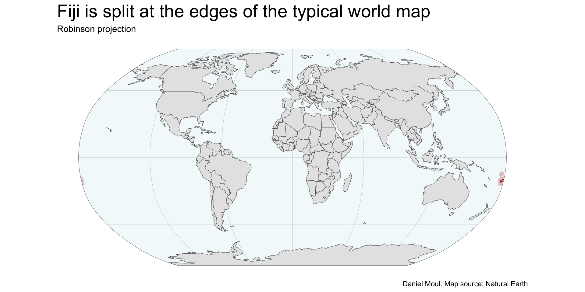
The Fiji Islands are so small and remote from the major continents that they are often omitted from world maps, or when they are included, relegated to the edges of the map, since Fiji land masses are just west and east of 180°:

Show the code
world = ne_countries()

world_robin <- world |>
  st_transform(crs = my_proj)

fiji = ne_countries(country = "Fiji", returnclass = "sf", scale = "large") |>
  st_wrap_dateline(options = c("WRAPDATELINE=YES", "DATELINEOFFSET=30"), quiet = TRUE)

fiji_bbox <- st_bbox(fiji)
fiji_bbox["xmin"] <- 177
my_fiji_crop <- fiji_bbox
fiji_cropped <- st_crop(fiji, my_fiji_crop)

fiji_buf <- st_buffer(fiji_cropped |>
                        st_transform(crs = "WGS84"), 
                      dist = 2) |>
  st_wrap_dateline(options = c("WRAPDATELINE=YES", "DATELINEOFFSET=1"), quiet = TRUE) |>
    st_transform(crs = my_proj)
# plot(fiji_buf$geometry)

grat <- st_graticule(x = c(-180, -90, 180, 90),
                     crs = "WGS84") |>
  st_transform(crs = my_proj)

# create water polygon for background 
lats <- c(90:-90, -90:90, 90)
longs <- c(rep(c(180, -180), each = 181), 180)
water_outline <- 
  list(cbind(longs, lats)) %>%
  st_polygon() %>%
  st_sfc(crs = "+proj=longlat +ellps=WGS84 +datum=WGS84 +no_defs") %>% 
  st_sf() %>%
  st_transform(crs = my_proj)

ggplot() +
  geom_sf(data = water_outline,
          fill = "lightblue", 
          linewidth = 0.15, alpha = 0.15
          ) +
  geom_sf(data = grat,
          fill = "lightblue", 
          linewidth = 0.15, alpha = 0.25) +
  geom_sf(data = world_robin) +
  geom_sf(data = fiji_buf, fill = "firebrick", color = NA, alpha = 0.25) +
  geom_sf(data = fiji_cropped, color = "firebrick", fill = "firebrick") +
  coord_sf(crs = my_proj) +
  theme(panel.border = element_blank()) +
  labs(
    title = "Fiji is split at the edges of the typical world map",
    subtitle = "Robinson projection",
    caption = "Daniel Moul. Map source: Natural Earth"
  )
Figure 1.1: World map (Robinson projection) splits Fiji at 180° longitude

1.1 PICT land and water area

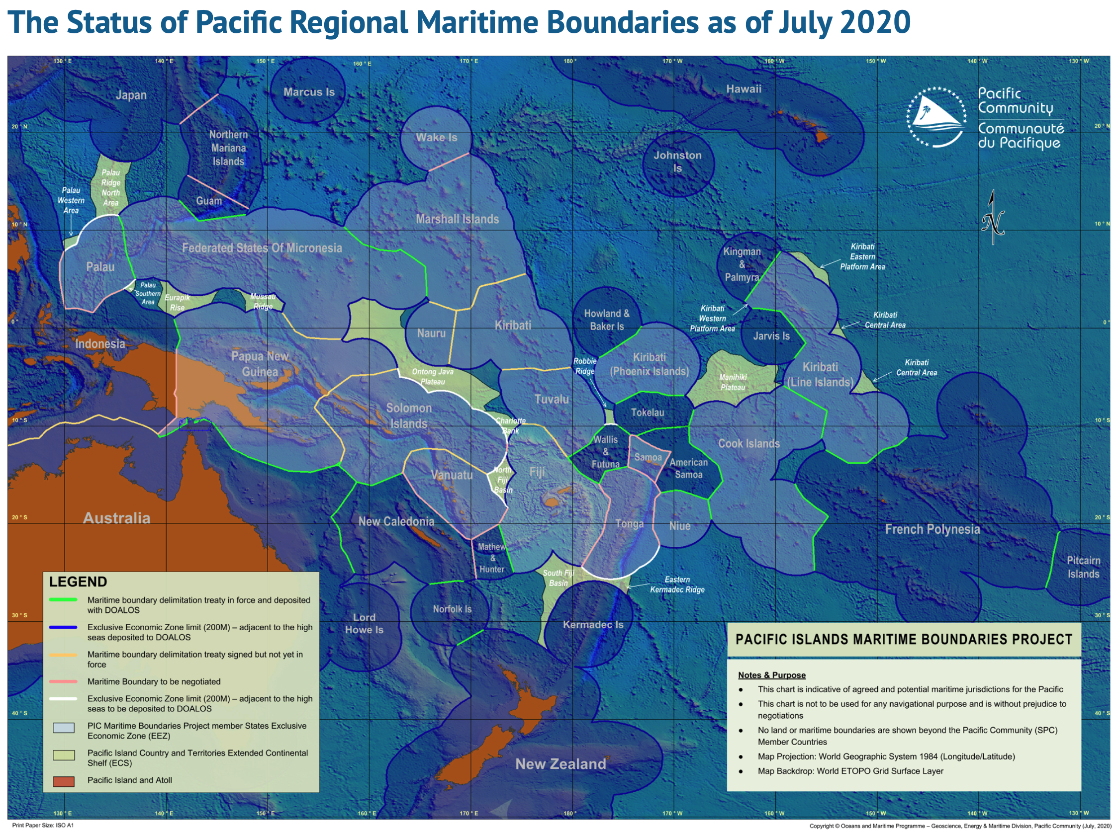
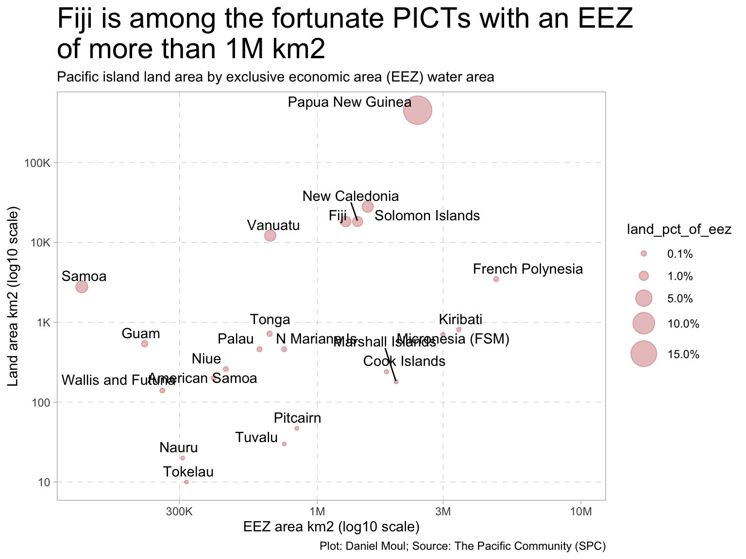
Like many other Pacific island countries and territories, there is an extensive exclusive economic zone (EEZ) surrounding the Fiji Islands:

Show the code
knitr::include_graphics(here("images/status-pacific-maritime-boundaries-spc-2020.png"))
Figure 1.2: Status of maritime boundaries July 20201
Show the code
d_pocket <- read_csv(here("./data/raw/pocket-summary/SPC_DF_POCKET_3.0_all.csv"),
               show_col_types = FALSE) |>
  clean_names() |>
  remove_empty(which = "cols") |>
  remove_constant() |>
  # rename(place = pacific_island_countries_and_territories) |>
  mutate(place = case_match(
    pacific_island_countries_and_territories,
    "Micronesia (Federated States of)"  ~ "Micronesia (FSM)",
    "Northern Mariana Islands"          ~ "N Mariana Is",
    .default = pacific_island_countries_and_territories
  ))

The the land area and Exclusive Economic Zone (EEZ) in the surrounding ocean varies widely among the PICTs.

Show the code
d_area_eez <- d_pocket |>
  filter(indicator_2 %in% c("Land area", "EEZ area")) |>
  arrange(desc(time_period)) |>
  distinct(geo_pict, indicator_2, .keep_all = TRUE) |>
  select(-c(time_period, unit_mult, unit_multiplier, data_year)) |>
  pivot_wider(id_cols = c(geo_pict, place), 
              names_from = indicator_2, values_from = obs_value) |>
  clean_names() |>
  mutate(land_pct_of_eez = land_area / eez_area)

d_area_eez |>
  ggplot(aes(eez_area, land_area)) +
  geom_vline(xintercept = c(3e5, 1e6, 3e6),
             lty = 2, linewidth = 0.15, alpha = 0.3) +
  geom_hline(yintercept = 10^c(1:5),
             lty = 2, linewidth = 0.15, alpha = 0.3) +
  geom_point(aes(size = land_pct_of_eez), 
             color = "firebrick", alpha = 0.3) +
  geom_text_repel(aes(label = place),
            hjust = 0, vjust = 1) +
  scale_x_log10(labels = label_number(scale_cut = cut_short_scale()),
                ) +
  scale_y_log10(labels = label_number(scale_cut = cut_short_scale())) +
  scale_size_continuous(range = c(1, 10),
                        labels = percent,
                        breaks = c(0.001, 0.01, 0.05, 0.1, 0.15)) +
  expand_limits(x = 1e7) +
  labs(
    title = "Fiji is among the fortunate PICTs with an EEZ\nof more than 1M km2",
    subtitle = "Pacific island land area by exclusive economic area (EEZ) water area",
    x = "EEZ area km2 (log10 scale)",
    y = "Land area km2 (log10 scale)",
    caption = my_caption
  )
Figure 1.3: Fiji is among the fortunate PICTs with an EEZ of more than 1M km2


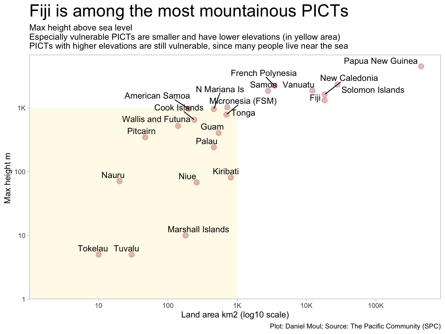
Some PICTs don’t rise much above sea level, others are mountainous.

Show the code
d_area_height <- d_pocket |>
  filter(indicator_2 %in% c("Land area", "Max height above sea level")) |>
  arrange(desc(time_period)) |>
  distinct(geo_pict, indicator_2, .keep_all = TRUE) |>
  select(-c(time_period, unit_mult, unit_multiplier, data_year)) |>
  pivot_wider(id_cols = c(geo_pict, place), 
              names_from = indicator_2, values_from = obs_value) |>
  clean_names()

d_area_height |>
  ggplot(aes(land_area, max_height_above_sea_level)) +
  annotate("rect", ymin = 1, ymax = 1000, xmin = 1, xmax = 1000,
           fill = "gold", alpha = 0.1) +
  # geom_vline(xintercept = 10^c(1:5),
  #            lty = 2, linewidth = 0.15, alpha = 0.3) +
  geom_point(size = 3,
             color = "firebrick", alpha = 0.3) +
  geom_text_repel(aes(label = place),
                  force = 2,
                  hjust = 0, vjust = 1) +
  scale_x_log10(labels = label_number(scale_cut = cut_short_scale()),
                expand = expansion(mult = c(0, 0.05)),
                breaks = 10^c(1:5)
  ) +
  scale_y_log10(labels = label_number(scale_cut = cut_short_scale()),
                expand = expansion(mult = c(0, 0.05))) +
  labs(
    title = "Fiji is among the most mountainous PICTs", 
    subtitle = glue("Max height above sea level",
                    "\nEspecially vulnerable PICTs are smaller and have lower elevations (in yellow area)",
                    "\nPICTs with higher elevations are still vulnerable, since many people live near the sea"),
    y = "Max height m ",
    x = "Land area km2 (log10 scale)",
    caption = my_caption
  )
Figure 1.4: Fiji is among the most mountainous PICTs


1.2 Focus on Fiji

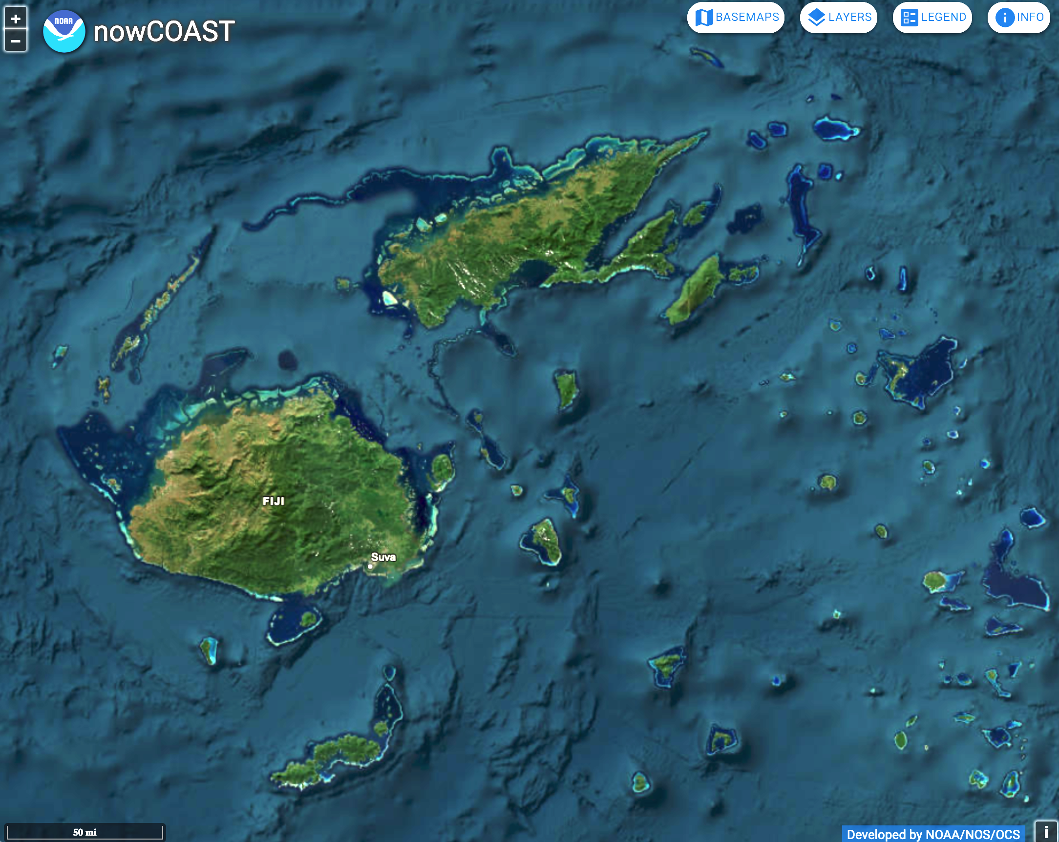
Fiji consists of more than 300 islands (more at low tide!). About three quarters of the people live on the main island Vitu Levu. The capital Suva is in the southeast, and the international airport Nadi (pronounced “nandi”) is in the west.

Show the code
knitr::include_graphics(here("images/fiji-zoomed-out-nowcoast-satellite-2024-06-22-lightened.png"))
Figure 1.5: Satellite image and bathymetry of most of the Fiji islands2


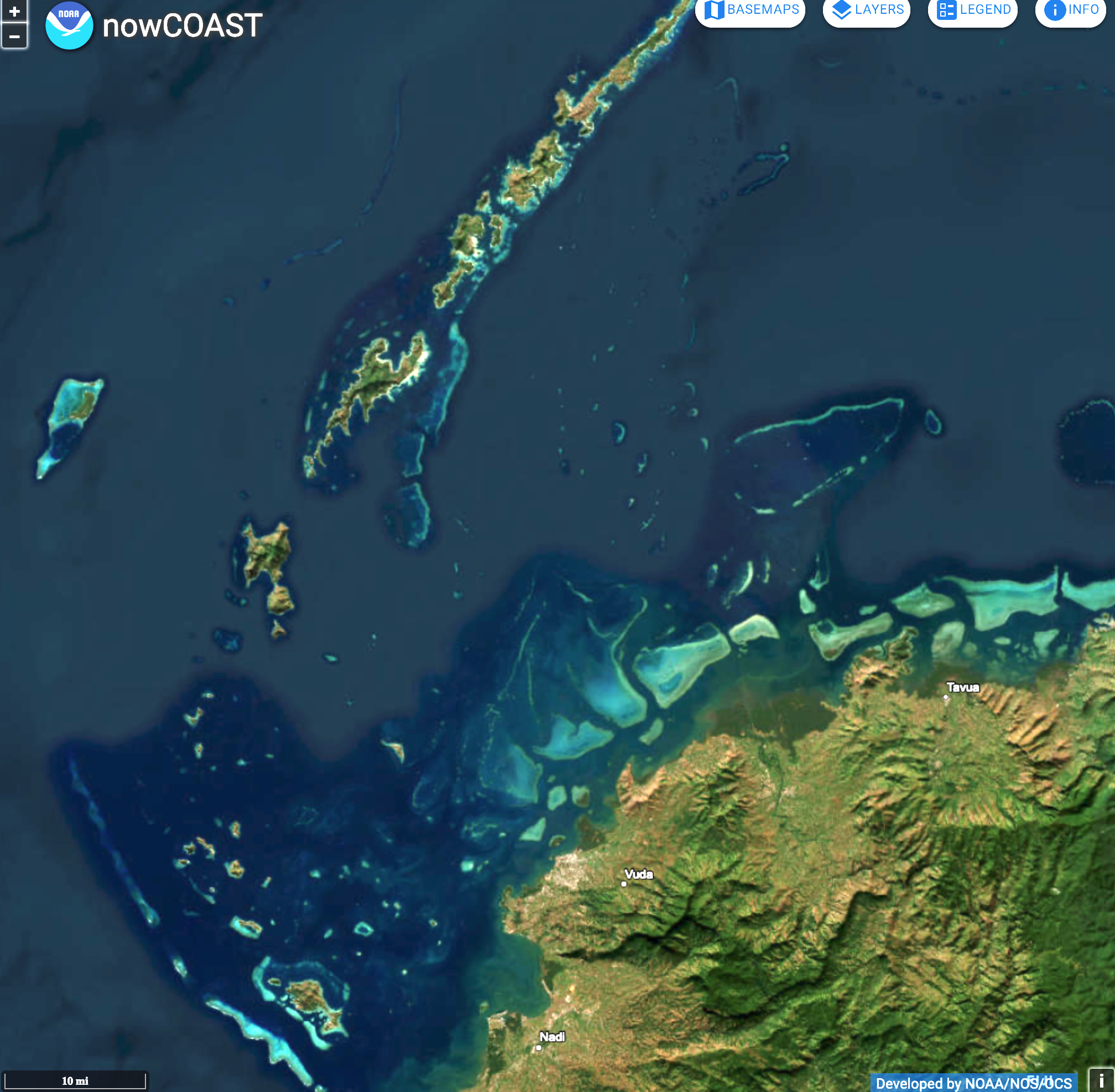
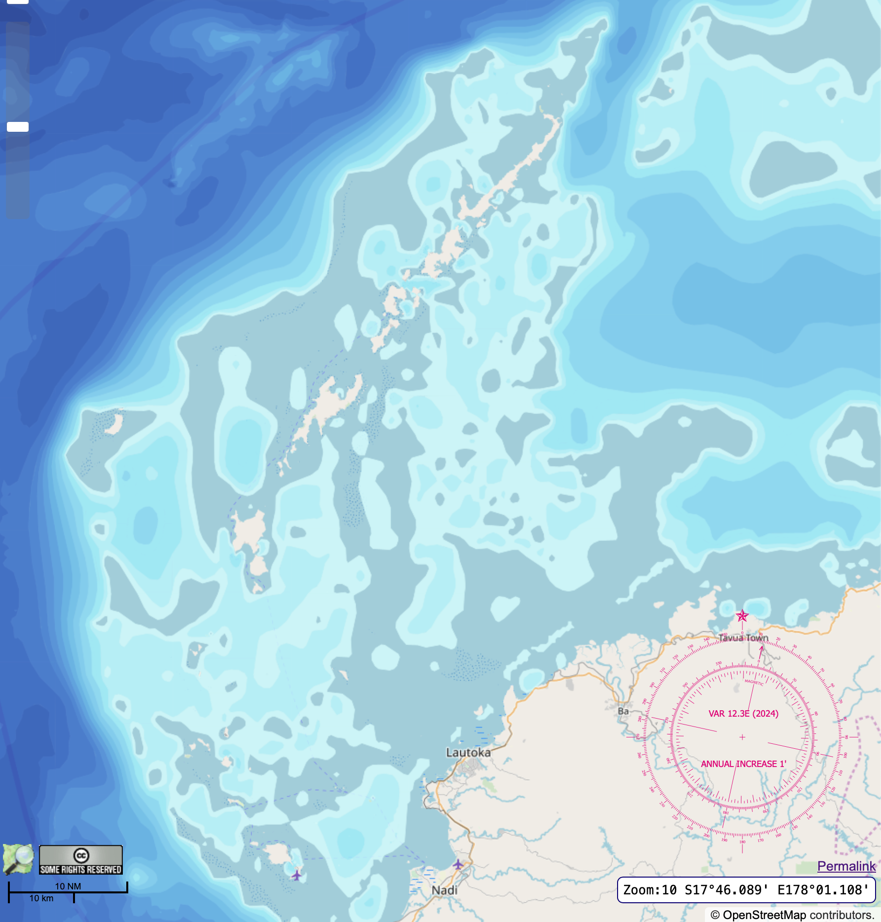
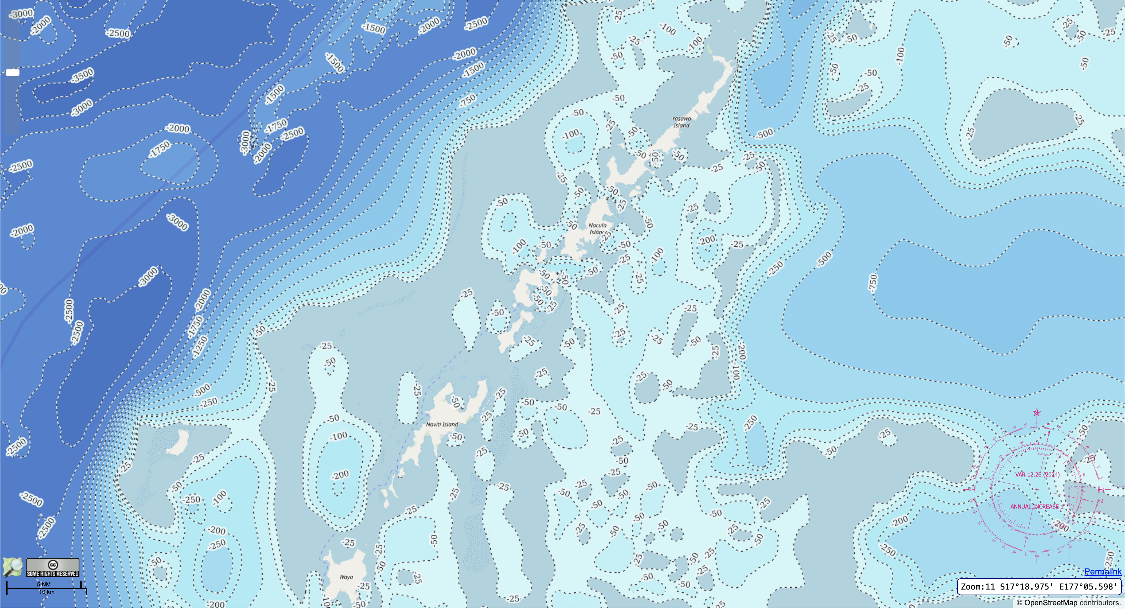
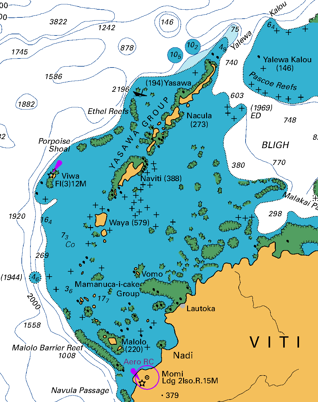
Most visitors coming for a holiday to Fiji arrive at Nadi airport on the western side of Viti Levu and stay nearby, since this area generally has the best weather, picturesque South Seas islands, and is easily accessible. The Mamanucas are the island group closest to Nadi, further north are the Yasawas.

Since my travels include the Yasawas, I focus below on the area between Nadi and the Yasawas.

Show the code
knitr::include_graphics(here("images/fiji-yasawas-mamanuthas-nowcoast-satellite-2024-06-22-lightened.png"))
Figure 1.6: Visual satellite image of western Viti Levu, the Mamanucas, and the Yawawas3


The water in this area is relatively shallow and interspersed with reefs. To the northwest of the Yasawas the shelf drops off quickly.

Show the code
###### GEBCO bathymetry grid2023

fj_file1 <- here("data/raw/GEBCO_22_Jun_2024_4b31746b7734/gebco_2023_n-16.6484_s-17.8168_w177.0208_e178.1079.tif")

fj_bath <- terra::rast(here(fj_file1)) |>
  rename(elev = `gebco_2023_n-16.6484_s-17.8168_w177.0208_e178.1079`)

my_bbox <- st_bbox(fj_bath)
# my_bbox_ext <- ext(fj_bath)

fj_bath_spatraster <- as_spatraster(fj_bath) |>
  mutate(elev = if_else(elev >= 0,
                        NA,
                        elev)) |>
  mutate(depth = -1 * elev) |>
  crop(coastline$osm_points)

bbox_spat <- ext(fj_bath_spatraster)
# SpatExtent : 177.029166666667, 178.108333333333, -17.8166666666667, -16.65 (xmin, xmax, ymin, ymax)
Show the code
plot_alpha <- 0.8

ggplot() +
  geom_spatraster_contour_filled(data = fj_bath_spatraster |>
                                   select(-1),
                          breaks = c(1, 5, 25, 50, 75, 150, 300, 1000, 2000, 3000, 4000),
                          , alpha = plot_alpha,
                          na.rm = TRUE) +
  geom_sf(data = coastline$osm_points,
          color = "brown", fill = "brown", size = 0.001, alpha = plot_alpha) +
  # geom_sf(data = islands$osm_polygons,
  #         color = "brown", fill = "brown", linewidth = 0.001, alpha = plot_alpha) +
  geom_sf(data = islands$osm_multipolygons,
          color = "brown", fill = "brown", linewidth = 0.001, alpha = plot_alpha) +
  geom_sf(data = coastline$osm_polygons,
          color = "brown", fill = "brown", linewidth = 0.001, alpha = plot_alpha) +
  # geom_sf(data = coastline$osm_polygons,
  #         color = "brown", fill = "brown", size = 0.001, alpha = plot_alpha) +
  coord_sf(xlim = bbox_spat[c(1, 2)], # min & max of x values
           ylim = bbox_spat[c(3, 4)]) +
  scale_x_continuous(expand = expansion(mult = c(0,0))) +
  scale_y_continuous(expand = expansion(mult = c(0,0))) +
  # scale_fill_viridis_d(direction = -1,
  #                      na.value = "transparent") +
  tidyterra::scale_fill_hypso_tint_d(palette = "etopo1_bathy",
                                     direction = -1) +
  guides(fill = guide_legend(reverse = FALSE,
                             position = "inside",
                             ncol = 2)) +
  theme(panel.background = element_rect(fill = "#F5DEB3"), 
        # "#FFFACD99"), # Doesn't seem panel.background honors alpha suffix "99"
        legend.position.inside = c(0.8, 0.15),
        axis.text = element_blank(),
        axis.ticks = element_blank()) +
  labs(
    title = "Bathymetry of the Yasawas, Mamanucas,\nand northwestern Viti Levu",
    subtitle = "Brown areas are land; cream-colored areas are shallows and reefs\nthat in some cases reach to sea level",
    caption = "Plot: Daniel Moul. Data: land masses from OSM, bathymetry from GEBCO Grid2023",
    fill = "Depth (m)"
  )

Bathymetry of the Yasawas, Mamanucas, and northwestern Viti Levu


The drop-off is more visible in the color scheme used by the Open Sea Map:

Show the code
knitr::include_graphics(here("images/western-fiji-yasawas-openseamap-2024-06-22.png"))
Figure 1.7: Western Viti Levu and the Yasawa islands: Open Sea Map with depths in meters4 based on data from Open Street Map.


Zooming in on the Yasawas:

Show the code
knitr::include_graphics(here("images/fiji-yasawas-closeup-openseamap-2024-06-07.png"))
Figure 1.8: Yasawa islands: Open Sea Map with depths in meters5 based on data from Open Street Map.


Marine charts represent this information differently:

Show the code
knitr::include_graphics(here("images/western-fiji-yasawas-land-info-nz-2020.png"))
Figure 1.9: Western Fiji including the Yasawa islands6


  1. GEM, Pacific Community https://gem.spc.int/news/2020/09/the-status-of-pacific-regional-maritime-boundaries-as-of-july-2020 ↩︎

  2. NOAA nowCOAST 2024-06-22 https://nowcoast.noaa.gov ↩︎

  3. NOAA nowCOAST 2024-06-22 https://nowcoast.noaa.gov ↩︎

  4. Openseamap.org https://map.openseamap.org/?zoom=9.9&lon=177.40986&lat=-17.15530&layers=TFFFFTFFFFFFFFFFTFFFFF ↩︎

  5. Openseamap.org https://map.openseamap.org/?zoom=10.9&lon=177.38484&lat=-16.95830&layers=TFFFFTFFFFFFFFFFTFFFFF ↩︎

  6. Western Fiji including the Yasawa islands Land Information NZ July 2020 NZ 14638 Fiji to Kermadec Islands including Tongatapu INT number 638 Scale 1:1500000 https://data.linz.govt.nz/layer/51355-chart-nz-14638-fiji-to-kermadec-islands-including-tongatapu/ ↩︎