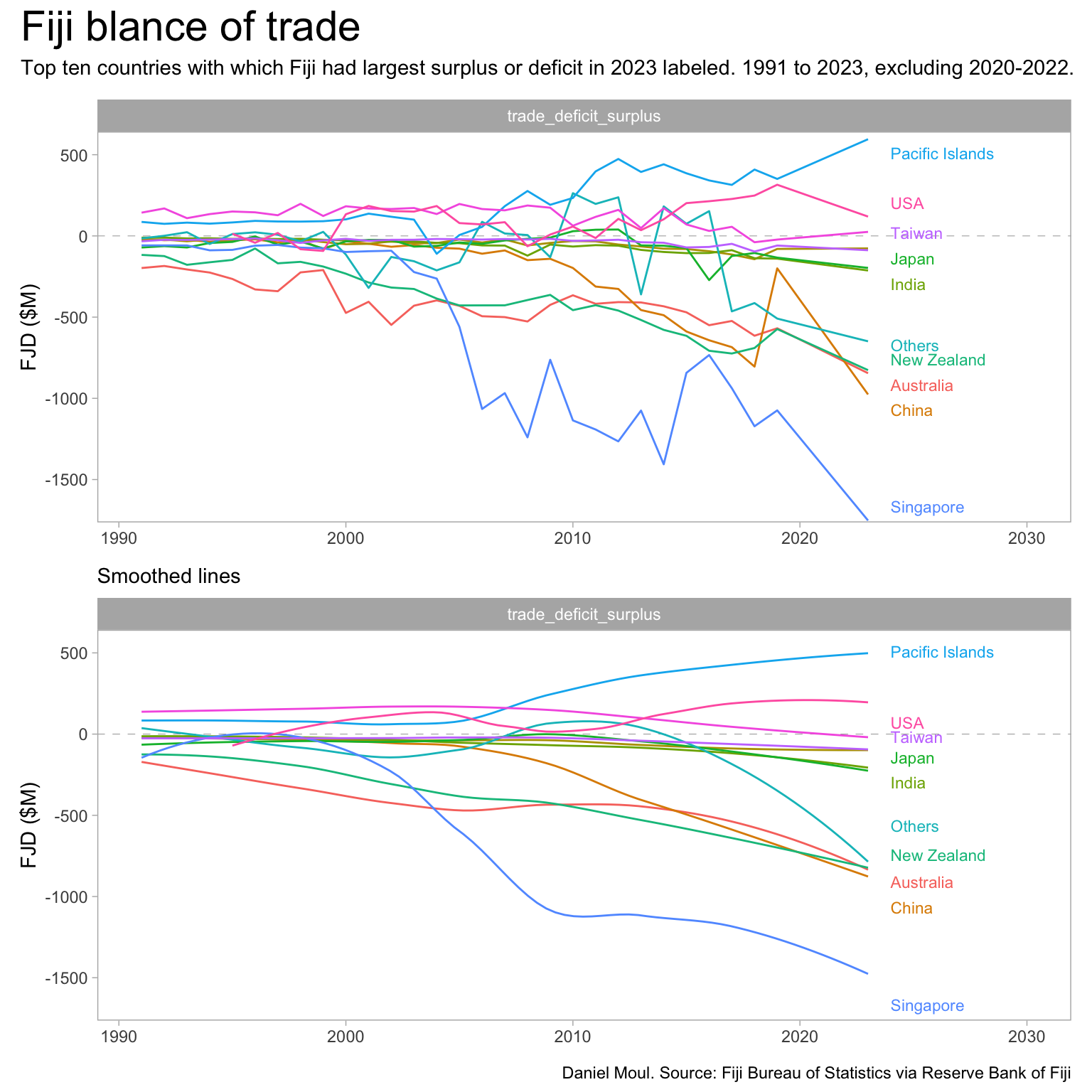
8  Exports, Imports and Balance of Trade

Show the code
source(here::here("scripts/load-libraries.R"))

theme_set(theme_light() +
            theme(panel.grid.major = element_blank(),
                  panel.grid.minor = element_blank(),
                  plot.title = element_text(size = rel(2))))

my_caption_rbf = "Daniel Moul. Source: Reserve Bank of Fiji"
my_caption_fbos = "Daniel Moul. Source: Fiji Bureau of Statistics via Reserve Bank of Fiji"

The Reserve Bank of Fiji provides the data used in this chapter.

Show the code
trade <- read_xlsx(here("data/raw/rbf/8.4-Direction-of-Trade-by-Major-Trading-Partner.xlsx"),
                   sheet = "Sheet1",
                   skip = 5) |>
  clean_names() |>
  remove_empty(which = c("rows", "cols")) |>
  filter(row_number() > 1) |>
  fill(country, .direction = "down") |>
  mutate(country = case_match(
    country,
    "China, Peoples Republic"           ~ "China",
    "China, Taiwan"                     ~ "Taiwan",
    "Germany, Federal"                  ~ "Germany",
    "Others & Other Asian Countries2/"  ~ "Others",
    .default = country
    ),
    across(year:trade_deficit_surplus, as.numeric),
    domestic_imports = imports - re_exports,
    domestic_imports = if_else(domestic_imports >= 0,
                               domestic_imports,
                               NA_real_)
    )

trade_year_min <- min(trade$year)
trade_year_max <- max(trade$year)

dta_for_plot_all <- trade |>
  filter(country != "TOTAL",
         country != "Germany", # omit, since not enough trade to be interesting
         !year %in% c(2020, 2021, 2022)) |>
  pivot_longer(domestic_exports:domestic_imports,
               names_to = "metric",
               values_to = "value")


8.1 Exports

Show the code
dta_for_plot <- dta_for_plot_all |>
  filter(metric %in% c("domestic_exports", "re_exports") ) 

dta_for_plot_labels <- dta_for_plot |>
  filter(year == 2023) |>
  group_by(metric) |>
  slice_max(order_by = abs(value),
            n = 5) |>
  ungroup() |>
  select(country, metric) |>
  mutate(country_label = country)

p1 <- dta_for_plot |>
  left_join(
    dta_for_plot_labels,
    by = c("country", "metric")
  ) |>
  ggplot(aes(year, value, color = country, group = country)) +
  geom_line(
    linewidth = 0.5,
    na.rm = TRUE,
    show.legend = FALSE
  ) +
  geom_text_repel(aes(x = 2024, 
                y = if_else(year == 2023,
                            value,
                            NA_real_), 
                label = country_label),
            size = 3, hjust = 0,
            direction = "y",
            na.rm = TRUE,
            show.legend = FALSE) +
  scale_y_continuous(expand = expansion(mult = c(0.005, 0.02))) +
  expand_limits(x = 2030) +
  facet_wrap(~ metric) +
  labs(
    x = NULL,
    y = "FJD ($M)"
  )

p2 <- dta_for_plot |>
  left_join(
    dta_for_plot_labels,
    by = c("country", "metric")
  ) |>
  ggplot(aes(year, value, color = country, group = country)) +
  geom_smooth(
    linewidth = 0.5,
    se = FALSE, method = 'loess', formula = 'y ~ x',
    na.rm = TRUE,
    show.legend = FALSE
  ) +
  geom_text_repel(aes(x = 2024, 
                y = if_else(year == 2023,
                            value,
                            NA_real_), 
                label = country_label),
            size = 3, hjust = 0,
            direction = "y",
            na.rm = TRUE,
            show.legend = FALSE) +
  scale_y_continuous(expand = expansion(mult = c(0.005, 0.02))) +
  expand_limits(x = 2030) +
  facet_wrap(~ metric) +
  coord_cartesian(ylim = c(0, NA)) +
  labs(
    subtitle = "Smoothed lines",
    x = NULL,
    y = "FJD ($M)"
  )

p1 / p2 +
  plot_annotation(
    title = "Fiji exports",
    subtitle = glue("Top five countries in 2023 labeled for each metric.", 
                    " {trade_year_min} to {trade_year_max}, excluding 2020-2022."),
    caption = my_caption_fbos
  )
Figure 8.1: Fiji exports


Show the code
dta_for_plot <- dta_for_plot_all |>
  filter(metric %in% c("domestic_exports", "re_exports") ) |>
  mutate(country_facet = fct_reorder(country, -value, sum))

p1 <- dta_for_plot |>
  left_join(
    dta_for_plot_labels,
    by = c("country", "metric")
  ) |>
  ggplot(aes(year, value, color = metric, group = metric)) +
  geom_line(
    linewidth = 0.5,
    na.rm = TRUE,
    show.legend = TRUE
  ) +
  scale_y_continuous(expand = expansion(mult = c(0.005, 0.02))) +
  scale_color_viridis_d(end = 0.9, direction = 1) +
  guides(color = guide_legend(override.aes = list(linewidth = 3))) +
  facet_wrap(~ country_facet) +
  theme(legend.position = "top") +
  labs(
    x = NULL,
    y = "FJD ($M)",
    color = NULL
  )

p2 <- dta_for_plot |>
  ggplot(aes(year, value, color = metric, group = metric)) +
  geom_smooth(
    linewidth = 0.5,
    se = FALSE, method = 'loess', formula = 'y ~ x',
    na.rm = TRUE,
    show.legend = FALSE
  ) +
  guides(color = guide_legend(override.aes = list(linewidth = 3))) +
  scale_y_continuous(expand = expansion(mult = c(0.005, 0.02))) +
  scale_color_viridis_d(end = 0.9, direction = 1) +
  facet_wrap(~ country_facet) +
  coord_cartesian(ylim = c(0, NA)) +
  labs(
    subtitle = "Smoothed lines",
    x = NULL,
    y = "FJD ($M)",
    color = NULL
  )

p1 / p2 +
  plot_annotation(
    title = "Fiji exports faceted by country",
    subtitle = glue("{trade_year_min} to {trade_year_max}, excluding 2020-2022.", 
                    " Facets ordered by total exports over time period."),
    caption = my_caption_fbos
  )
Figure 8.2: Fiji exports faceted by country


Show the code
dta_for_plot <- dta_for_plot_all |>
  filter(metric %in% c("domestic_exports", "re_exports") ) |>
  mutate(country_facet = fct_reorder(country, -value, sum))

p1 <- dta_for_plot |>
  left_join(
    dta_for_plot_labels,
    by = c("country", "metric")
  ) |>
  ggplot(aes(year, value, color = metric, group = metric)) +
  geom_line(
    linewidth = 0.5,
    na.rm = TRUE,
    show.legend = TRUE
  ) +
  scale_y_continuous(expand = expansion(mult = c(0.005, 0.02))) +
  scale_color_viridis_d(end = 0.9, direction = 1) +
  guides(color = guide_legend(override.aes = list(linewidth = 3))) +
  facet_wrap(~ country_facet, scales = "free_y") +
  theme(legend.position = "top") +
  labs(
    x = NULL,
    y = "FJD ($M)",
    color = NULL
  )

p2 <- dta_for_plot |>
  ggplot(aes(year, value, color = metric, group = metric)) +
  geom_smooth(
    linewidth = 0.5,
    se = FALSE, method = 'loess', formula = 'y ~ x',
    na.rm = TRUE,
    show.legend = FALSE
  ) +
  guides(color = guide_legend(override.aes = list(linewidth = 3))) +
  scale_y_continuous(expand = expansion(mult = c(0.005, 0.02))) +
  scale_color_viridis_d(end = 0.9, direction = 1) +
  facet_wrap(~ country_facet, scales = "free_y") +
  coord_cartesian(ylim = c(0, NA)) +
  labs(
    subtitle = "Smoothed lines",
    x = NULL,
    y = "FJD ($M)",
    color = NULL
  )

p1 / p2 +
  plot_annotation(
    title = "Fiji exports faceted by country (Y axis scale varies)",
    subtitle = glue("{trade_year_min} to {trade_year_max}, excluding 2020-2022.",
                    " Facets ordered by total exports over time period."),
    caption = my_caption_fbos
  )
Figure 8.3: Fiji exports faceted by country (Y axis scale varies to make country-level trends more visible)


8.2 Imports

Show the code
dta_for_plot <- dta_for_plot_all |>
  filter(metric %in% c("domestic_imports", "imports") ) |>
  mutate(country_facet = fct_reorder(country, -value, sum))

p1 <- dta_for_plot |>
  left_join(
    dta_for_plot_labels,
    by = c("country", "metric")
  ) |>
  ggplot(aes(year, value, color = metric, group = metric)) +
  geom_line(
    linewidth = 0.5,
    na.rm = TRUE,
    show.legend = TRUE
  ) +
  scale_y_continuous(expand = expansion(mult = c(0.005, 0.02))) +
  scale_color_viridis_d(end = 0.9, direction = -1) +
  guides(color = guide_legend(override.aes = list(linewidth = 3))) +
  facet_wrap(~ country_facet) +
  theme(legend.position = "top") +
  labs(
    x = NULL,
    y = "FJD ($M)",
    color = NULL
  )

p2 <- dta_for_plot |>
  ggplot(aes(year, value, color = metric, group = metric)) +
  geom_smooth(
    linewidth = 0.5,
    se = FALSE, method = 'loess', formula = 'y ~ x',
    na.rm = TRUE,
    show.legend = FALSE
  ) +
  guides(color = guide_legend(override.aes = list(linewidth = 3))) +
  scale_y_continuous(expand = expansion(mult = c(0.005, 0.02))) +
  scale_color_viridis_d(end = 0.9, direction = -1) +
  facet_wrap(~ country_facet) +
  coord_cartesian(ylim = c(0, NA)) +
  labs(
    subtitle = "Smoothed lines",
    x = NULL,
    y = "FJD ($M)",
    color = NULL
  )

p1 / p2 +
  plot_annotation(
    title = "Fiji imports faceted by country",
    subtitle = glue("{trade_year_min} to {trade_year_max}, excluding 2020-2022.",
                    "\nFacets ordered by total imports over time period."),
    caption = my_caption_fbos
  )
Figure 8.4: Fiji imports faceted by country


Show the code
dta_for_plot <- dta_for_plot_all |>
  filter(metric %in% c("domestic_imports", "imports") ) |>
  mutate(country_facet = fct_reorder(country, -value, sum))

p1 <- dta_for_plot |>
  left_join(
    dta_for_plot_labels,
    by = c("country", "metric")
  ) |>
  ggplot(aes(year, value, color = metric, group = metric)) +
  geom_line(
    linewidth = 0.5,
    na.rm = TRUE,
    show.legend = TRUE
  ) +
  scale_y_continuous(expand = expansion(mult = c(0.005, 0.02))) +
  scale_color_viridis_d(end = 0.9, direction = -1) +
  guides(color = guide_legend(override.aes = list(linewidth = 3))) +
  expand_limits(y = 0) +
  facet_wrap(~ country_facet, scales = "free_y") +
  theme(legend.position = "top") +
  labs(
    x = NULL,
    y = "FJD ($M)",
    color = NULL
  )

p2 <- dta_for_plot |>
  ggplot(aes(year, value, color = metric, group = metric)) +
  geom_smooth(
    linewidth = 0.5,
    se = FALSE, method = 'loess', formula = 'y ~ x',
    na.rm = TRUE,
    show.legend = FALSE
  ) +
  guides(color = guide_legend(override.aes = list(linewidth = 3))) +
  scale_y_continuous(expand = expansion(mult = c(0.005, 0.02))) +
  scale_color_viridis_d(end = 0.9, direction = -1) +
  expand_limits(y = 0) +
  facet_wrap(~ country_facet, scales = "free_y") +
  coord_cartesian(ylim = c(0, NA)) +
  labs(
    subtitle = "Smoothed lines",
    x = NULL,
    y = "FJD ($M)",
    color = NULL
  )

p1 / p2 +
  plot_annotation(
    title = "Fiji imports faceted by country (Y axis scale varies)",
    subtitle = glue("{trade_year_min} to {trade_year_max}, excluding 2020-2022.",
                    " Facets ordered by total imports over time period."),
    caption = my_caption_fbos
  )
Figure 8.5: Fiji imports faceted by country (Y axis varies to make country-level trends more visible)


8.3 Balance of trade

Show the code
dta_for_plot <- dta_for_plot_all |>
  filter(metric %in% c("trade_deficit_surplus") ) 

dta_for_plot_labels <- dta_for_plot |>
  filter(year == 2023) |>
  group_by(metric) |>
  slice_max(order_by = abs(value),
            n = 10) |>
  ungroup() |>
  select(country, metric) |>
  mutate(country_label = country)

p1 <- dta_for_plot |>
  left_join(
    dta_for_plot_labels,
    by = c("country", "metric")
  ) |>
  ggplot(aes(year, value, color = country, group = country)) +
  geom_hline(yintercept = 0, lty = 2, linewidth = 0.15, alpha = 0.5) +
  geom_line(
    linewidth = 0.5,
    na.rm = TRUE,
    show.legend = FALSE
  ) +
  geom_text_repel(aes(x = 2024, 
                y = if_else(year == 2023,
                            value,
                            NA_real_), 
                label = country_label),
            size = 3, hjust = 0,
            direction = "y",
            na.rm = TRUE,
            show.legend = FALSE) +
  scale_y_continuous(expand = expansion(mult = c(0.005, 0.02))) +
  expand_limits(x = 2030) +
  facet_wrap(~ metric) +
  labs(
    x = NULL,
    y = "FJD ($M)"
  )

p2 <- dta_for_plot |>
  left_join(
    dta_for_plot_labels,
    by = c("country", "metric")
  ) |>
  ggplot(aes(year, value, color = country, group = country)) +
  geom_hline(yintercept = 0, lty = 2, linewidth = 0.15, alpha = 0.5) +
  geom_smooth(
    linewidth = 0.5,
    se = FALSE, method = 'loess', formula = 'y ~ x',
    na.rm = TRUE,
    show.legend = FALSE
  ) +
  geom_text_repel(aes(x = 2024, 
                y = if_else(year == 2023,
                            value,
                            NA_real_), 
                label = country_label),
            size = 3, hjust = 0,
            direction = "y",
            na.rm = TRUE,
            show.legend = FALSE) +
  scale_y_continuous(expand = expansion(mult = c(0.005, 0.02))) +
  expand_limits(x = 2030) +
  facet_wrap(~ metric) +
  labs(
    subtitle = "Smoothed lines",
    x = NULL,
    y = "FJD ($M)"
  )

p1 / p2 +
  plot_annotation(
    title = "Fiji blance of trade",
    subtitle = glue("Top ten countries with which Fiji had largest surplus or deficit in 2023 labeled.", 
                    " {trade_year_min} to {trade_year_max}, excluding 2020-2022."),
    caption = my_caption_fbos
  )
Figure 8.6: Fiji balance of trade


Show the code
dta_for_plot <- dta_for_plot_all |>
  filter(metric %in% c("trade_deficit_surplus") ) |>
  mutate(country_facet = fct_reorder(country, -value, sum))

p1 <- dta_for_plot |>
  # left_join(
  #   dta_for_plot_labels,
  #   by = c("country", "metric")
  # ) |>
  ggplot(aes(year, value, color = metric, group = metric)) +
  geom_hline(yintercept = 0, lty = 2, linewidth = 0.15, alpha = 0.5) +
  geom_line(
    linewidth = 0.5,
    na.rm = TRUE,
    show.legend = FALSE
  ) +
  scale_y_continuous(expand = expansion(mult = c(0.005, 0.02))) +
  guides(color = guide_legend(override.aes = list(linewidth = 3))) +
  facet_wrap(~ country_facet) +
  theme(legend.position = "top") +
  labs(
    x = NULL,
    y = "FJD ($M)"
  )

p2 <- dta_for_plot |>
  ggplot(aes(year, value, color = metric, group = metric)) +
  geom_hline(yintercept = 0, lty = 2, linewidth = 0.15, alpha = 0.5) +
  geom_smooth(
    linewidth = 0.5,
    se = FALSE, method = 'loess', formula = 'y ~ x',
    na.rm = TRUE,
    show.legend = FALSE
  ) +
  guides(color = guide_legend(override.aes = list(linewidth = 3))) +
  scale_y_continuous(expand = expansion(mult = c(0.005, 0.02))) +
  facet_wrap(~ country_facet) +
  labs(
    subtitle = "Smoothed lines",
    x = NULL,
    y = "FJD ($M)"
  )

p1 / p2 +
  plot_annotation(
    title = "Fiji balance of trade faceted by country",
    subtitle = glue("{trade_year_min} to {trade_year_max}, excluding 2020-2022.", 
                    " Facets ordered by sum of balance over time period."),
    caption = my_caption_fbos
  )
Figure 8.7: Fiji balance of trade faceted by country


Show the code
dta_for_plot <- dta_for_plot_all |>
  filter(metric %in% c("trade_deficit_surplus") ) |>
  mutate(country_facet = fct_reorder(country, -value, sum))

p1 <- dta_for_plot |>
  left_join(
    dta_for_plot_labels,
    by = c("country", "metric")
  ) |>
  ggplot(aes(year, value, color = metric, group = metric)) +
  geom_hline(yintercept = 0, lty = 2, linewidth = 0.15, alpha = 0.5) +
  geom_line(
    linewidth = 0.5,
    na.rm = TRUE,
    show.legend = FALSE
  ) +
  scale_y_continuous(expand = expansion(mult = c(0.005, 0.02))) +
  guides(color = guide_legend(override.aes = list(linewidth = 3))) +
  facet_wrap(~ country_facet, scales = "free_y") +
  theme(legend.position = "top") +
  labs(
    x = NULL,
    y = "FJD ($M)"
  )

p2 <- dta_for_plot |>
  ggplot(aes(year, value, color = metric, group = metric)) +
  geom_hline(yintercept = 0, lty = 2, linewidth = 0.15, alpha = 0.5) +
  geom_smooth(
    linewidth = 0.5,
    se = FALSE, method = 'loess', formula = 'y ~ x',
    na.rm = TRUE,
    show.legend = FALSE
  ) +
  guides(color = guide_legend(override.aes = list(linewidth = 3))) +
  scale_y_continuous(expand = expansion(mult = c(0.005, 0.02))) +
  facet_wrap(~ country_facet, scales = "free_y") +
  # coord_cartesian(ylim = c(0, NA)) +
  labs(
    subtitle = "Smoothed lines",
    x = NULL,
    y = "FJD ($M)"
  )

p1 / p2 +
  plot_annotation(
    title = "Fiji balance of trade faceted by country",
    subtitle = glue("{trade_year_min} to {trade_year_max}, excluding 2020-2022.",
                    " Facets ordered by sum of balance over time period."),
    caption = my_caption_fbos
  )
Figure 8.8: Fiji balance of trade faceted by country (Y axis varies to make country-level trends more visible)


8.4 General Notes

  • Differences from previously published tables are due to revisions.
  • Others includes France, Netherlands, Spain & Other Asian Countries (Indonesia, Korea, Malaysia, Thailand and Vietnam) from 2023 onwards.
  • Data for the years 2015, 2018, 2019, 2021 & 2023 have been revised.
  • Data for the year 2023 is provisional.

Daniel’s additional notes

  • domestic exports, re-exports, and total exports are F.O.B.
  • imports are C.I.F.
  • domestic imports are imports less re-exports
  • all amounts are nominal dollars FJD (not adjusted for inflation)